Business Intelligence Archives - SQL Freelancer Blog

SSIS Series: How to use Conditional Split

By bradyupton in Business Intelligence, Integration Services (SSIS), SSIS Series January 30, 2023 0 Comment

From Microsoft, the Conditional Split transformation can route data rows to different outputs depending on the content of the data. The implementation of the Conditional Split transformation is similar to a CASE decision structure in a programming language. The transformation evaluates expressions, and based on the results, directs the data row to the specified output. This transformation also provides a default output, so that if a row matches no expression it is directed to the default output.

You can configure the Conditional Split transformation in the following ways:

Provide an expression that evaluates to a Boolean for each condition you want the transformation to test.
Specify the order in which the conditions are evaluated. Order is significant, because a row is sent to the output corresponding to the first condition that evaluates to true.
Specify the default output for the transformation. The transformation requires that a default output be specified.

Let’s take a look at how this transformation might be used in the real world.

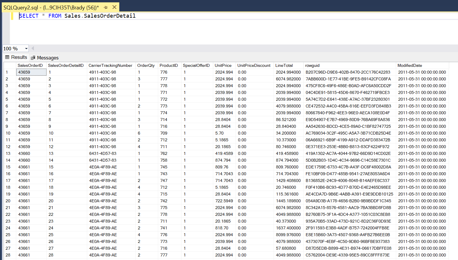
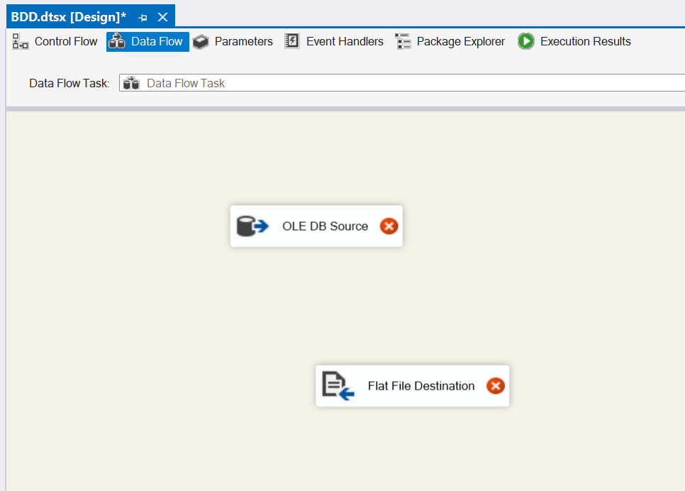
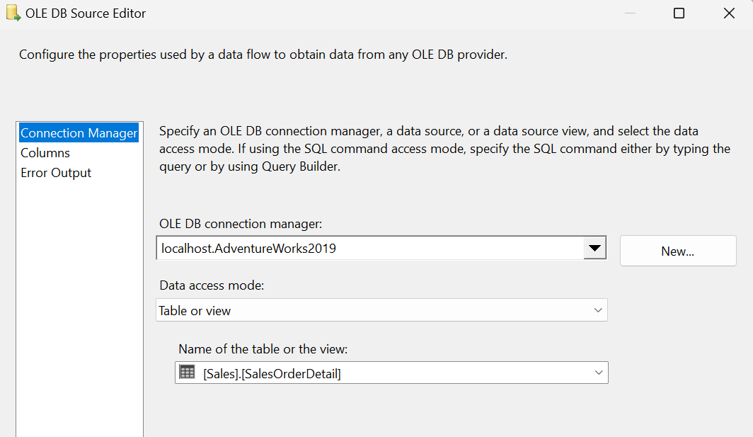
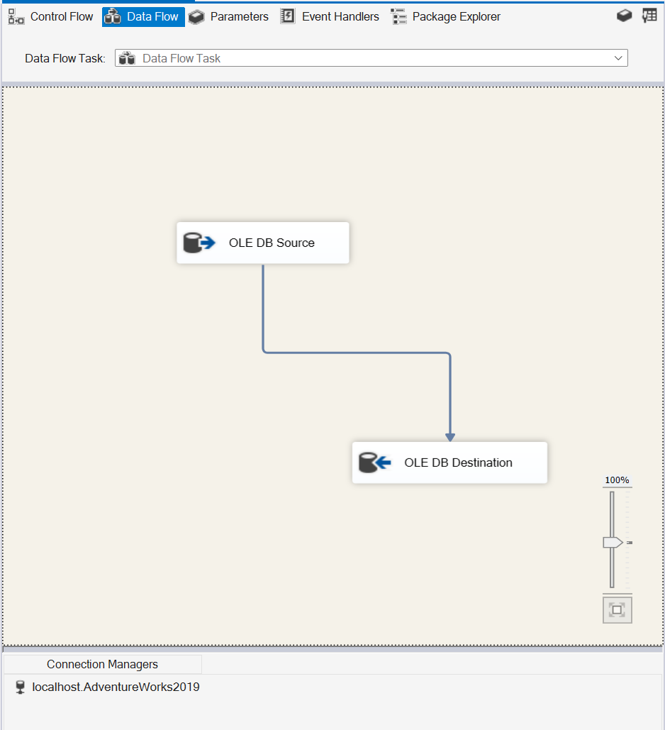
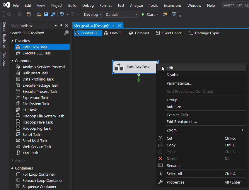
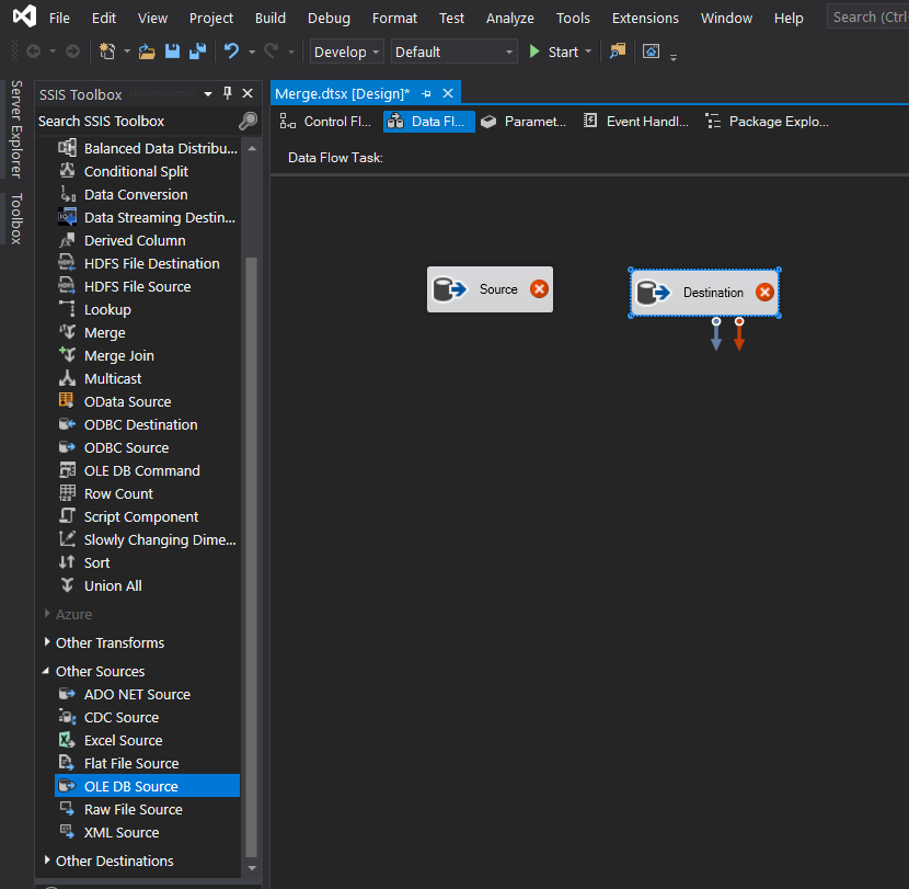
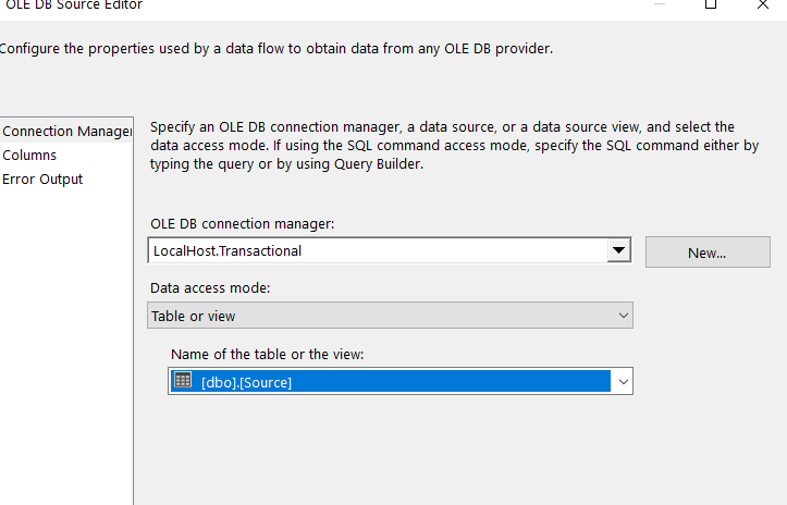
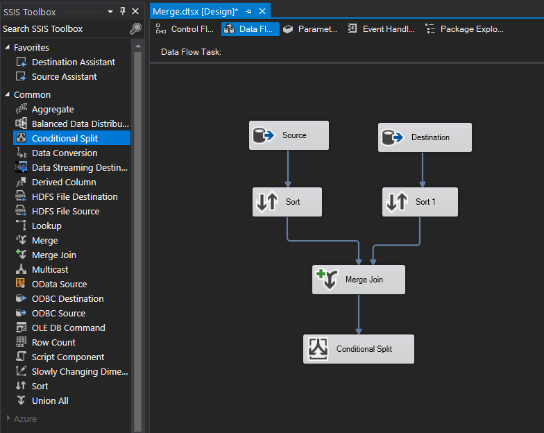
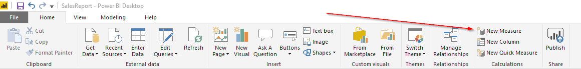
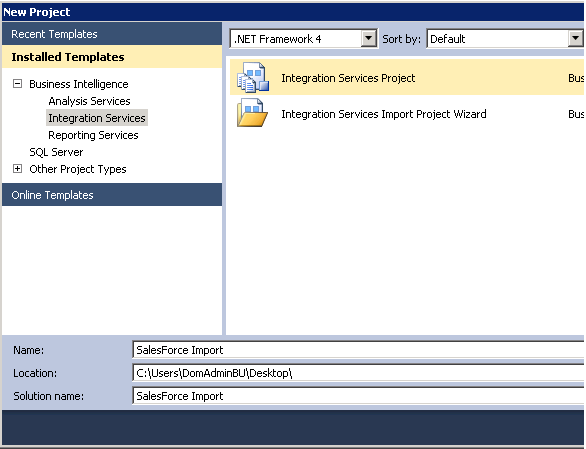
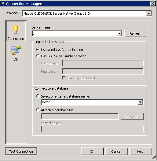
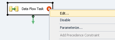
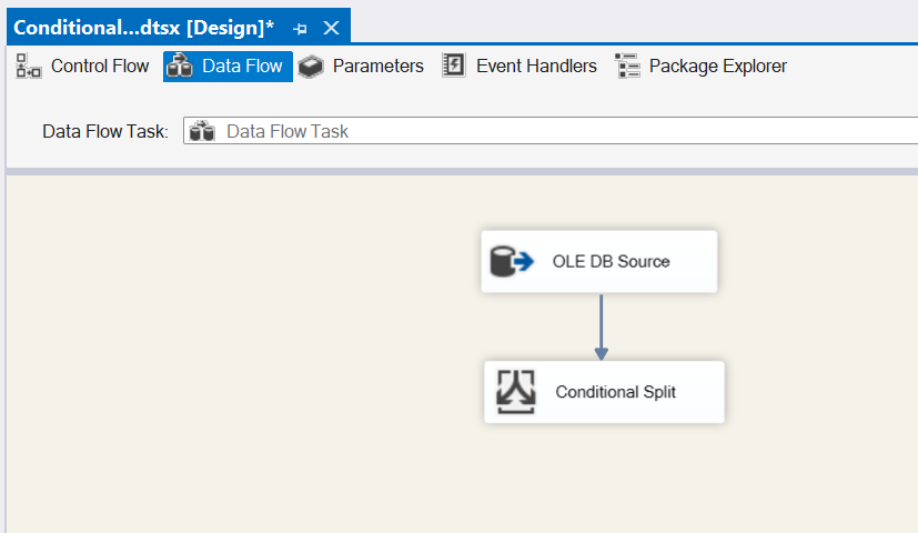
Open Visual Studio and drag a Data Flow task into the design pane. Open the Data Flow task and drag in an OLE DB Source task. For this post, I’m going to use the AdventureWorks2019 database and the HumanResources.vEmployeeDepartment view.

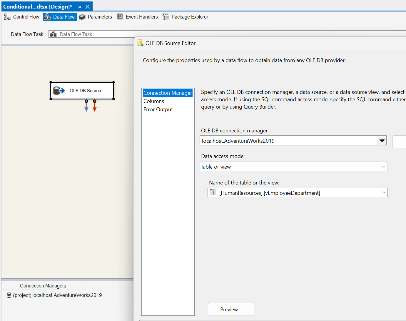
This view has some good data to play around with, but we’re going to focus on the Department and Start Date columns. Let’s pretend the bossman needs to see all of the Employees in the Quality Assurance (QA), Production and Sales Department in a separate database table. Bonus, he needs to see all of the Production employees split up into two more tables based on who started before and after Jan 1, 2010. All other employees can go into their own table. Got it? Great! That’s 5 total tables. QA=1, Production=2, Sales=1, Leftovers=1 Let’s go.

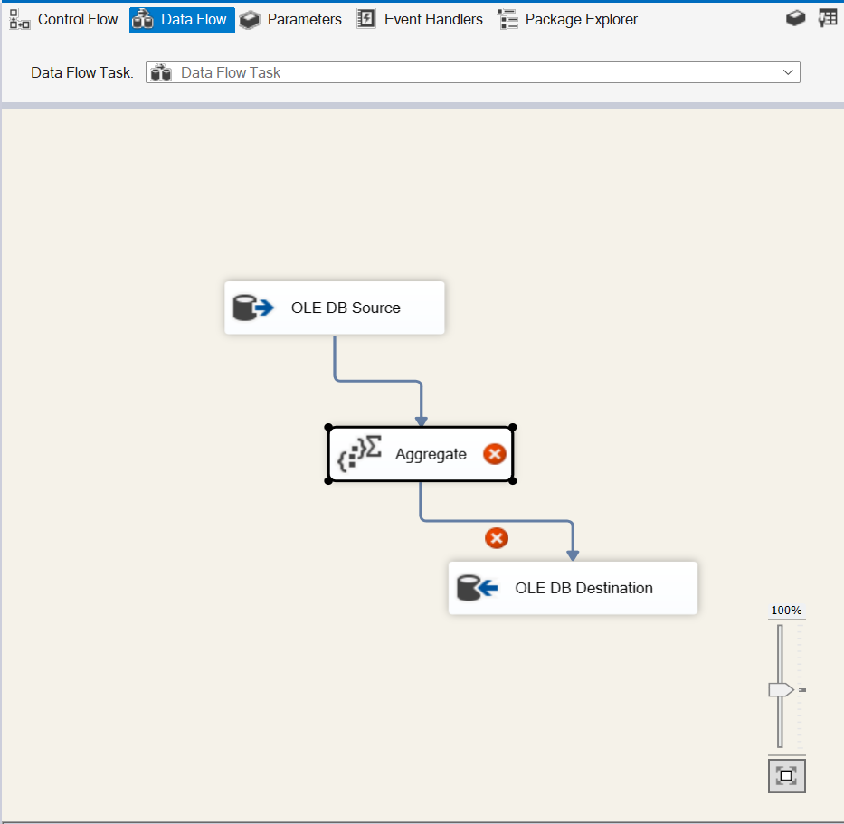
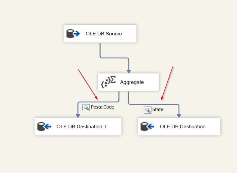
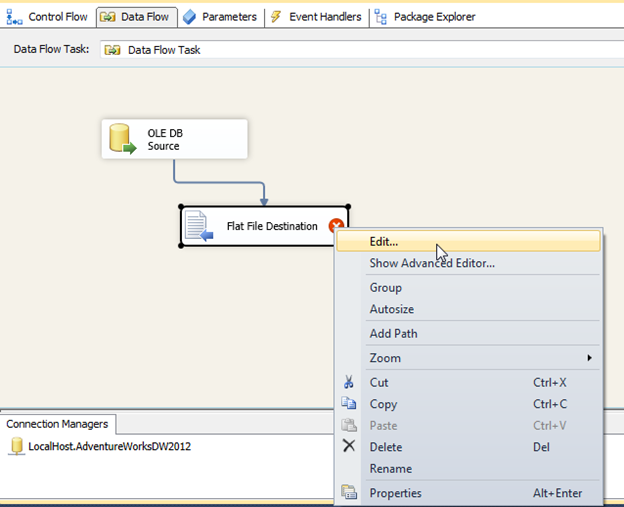
Back in Visual Studio, drag in a Conditional Split task and connect it to our OLE DB Source.

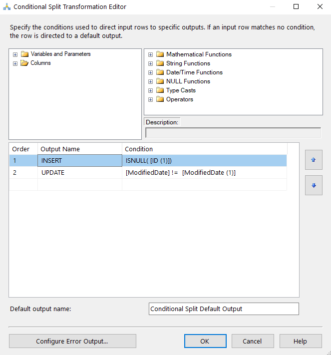
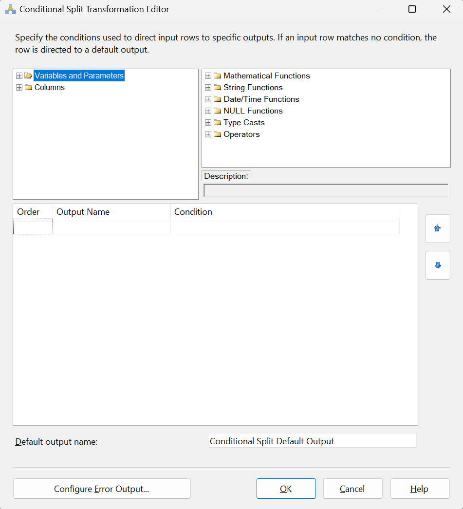
Open the Conditional Split task editor and you’ll see a few options (from left to right, top to bottom):

We can use columns and/or variables and parameters in our expressions that define how to split the data flow.
We can use functions such as Date/Time, NULL and String in our expressions that define how to split the data flow.
These are the conditions that define how to split the data flow. These need to be set in priority order; any rows that evaluate to true for one condition will not be available to the condition that follows.

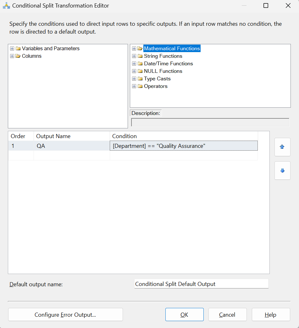
Let’s start adding some conditions for our data. First, we’ll add a condition for all of our QA Department Employees. I’ll name the output “QA” and my condition is pretty simple whereas Department == “Quality Assurance”.

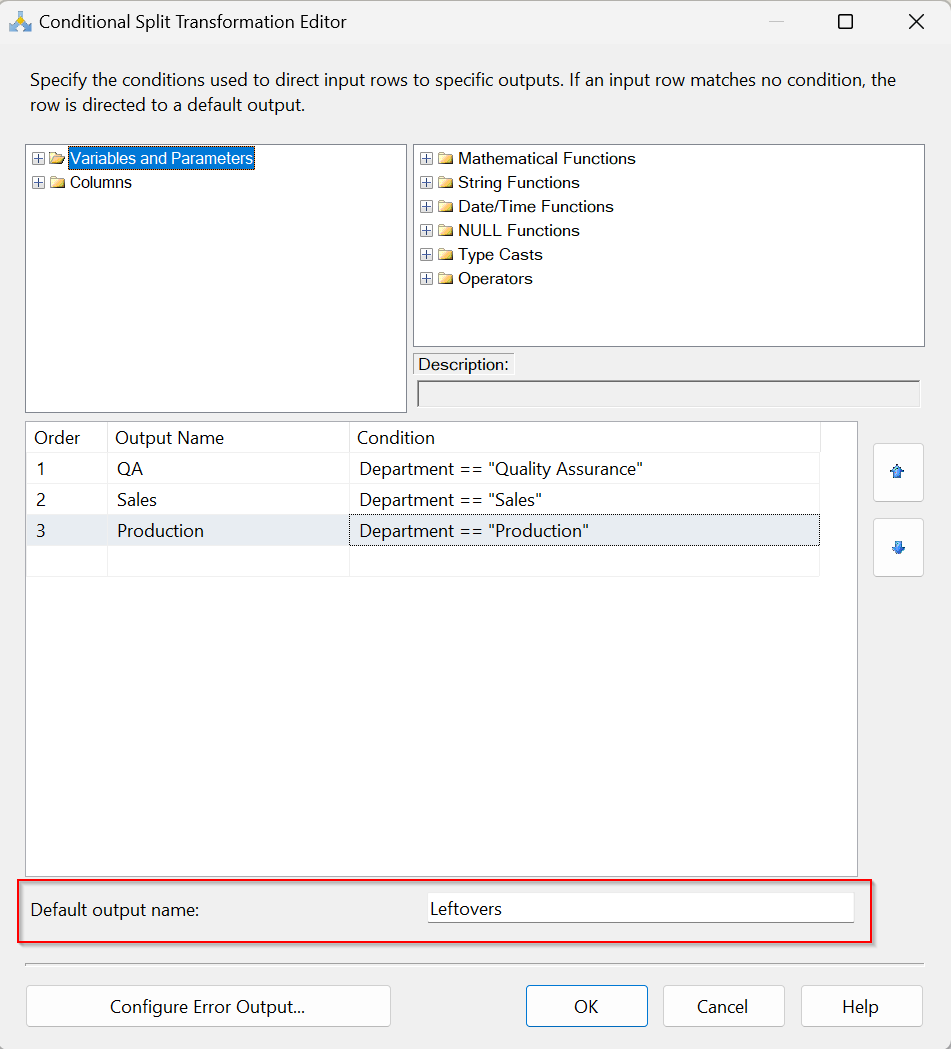
I’ll do the same for Production, Sales and Leftovers (everything else that doesn’t satisfy a condition). Since Leftovers is everything else we’ll just change the name of the Default Output name to identify it.

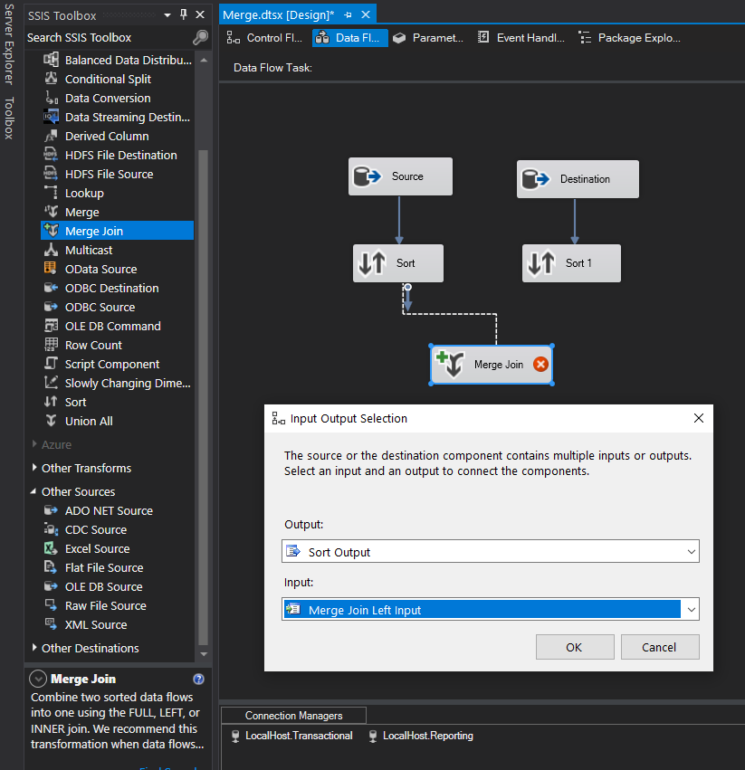
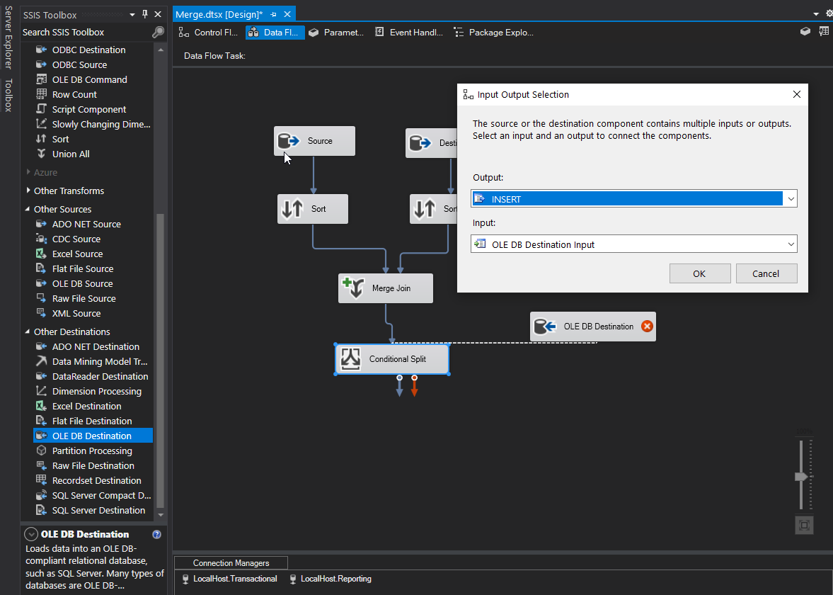
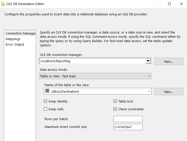
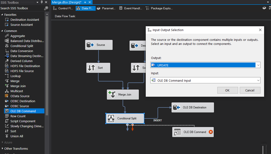
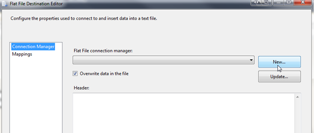
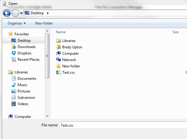
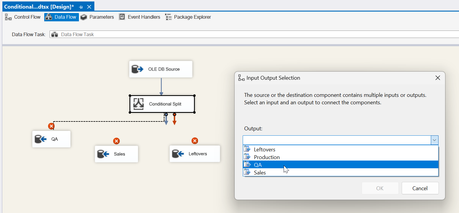
Let’s go ahead and add our destination tasks (except for Production since we need another condition) and link them to the appropriate condition. See below for QA as an example. When we drag our connector to our destination task we get prompted with an Input Output Selection box. Here is where we choose our Condition that will match up with our table. For the screenshot below, we’ll choose QA output for our QA destination.

Now that we have QA mapped, go ahead and map Sales and Leftovers.

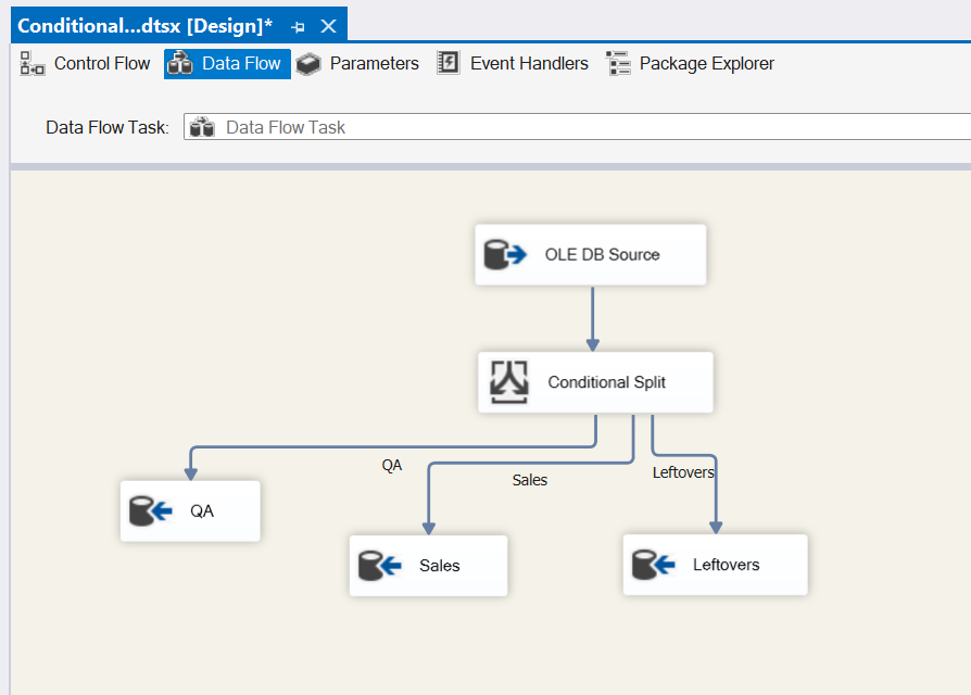
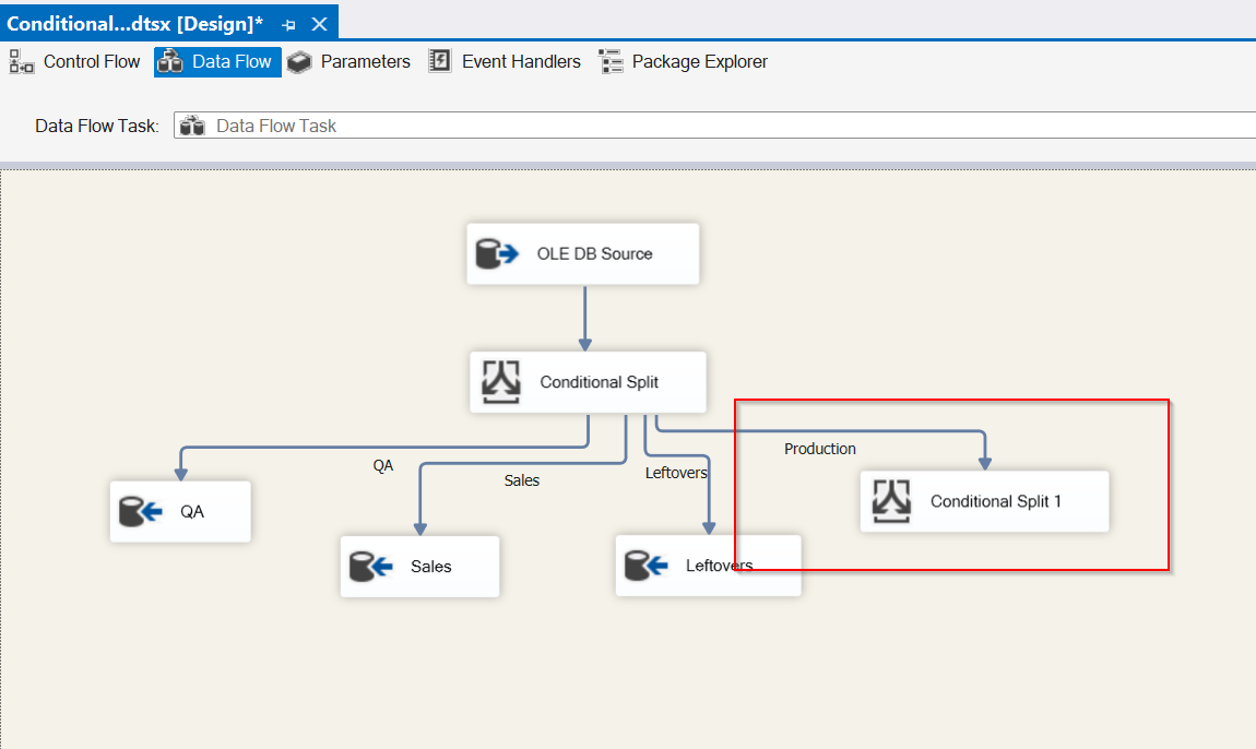
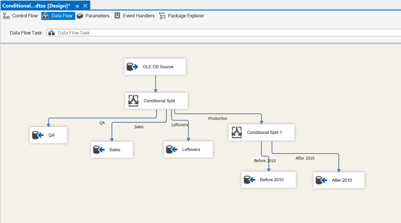
Looks great! QA, Sales and Leftovers are mapped successfully. Let’s take a look at adding another Conditional Split task for Production. Drag a Conditional Split task into the design pane and connect it to the current Conditional Split. It automatically maps to Production since it’s the only output left.

From our new Conditional split task, let’s open the editor and configure the date conditions for Production. We’ll leave the Default output name box as is since we shouldn’t have any leftover data from this split.

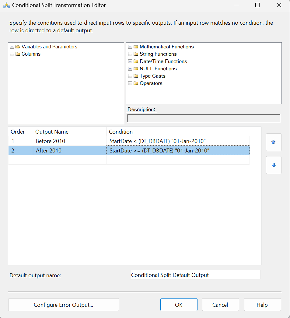
Now we can map the two new conditions to their appropriate destinations.

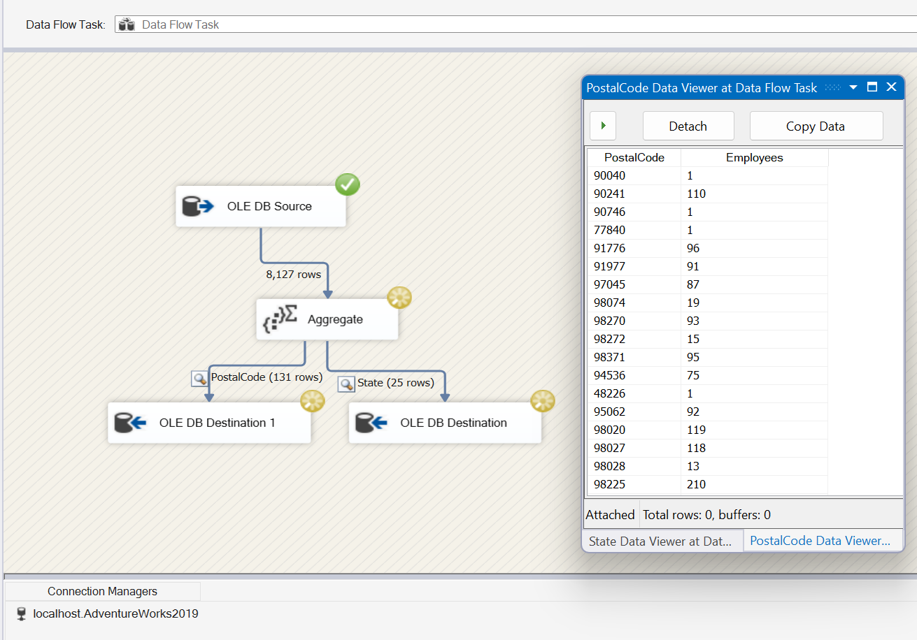
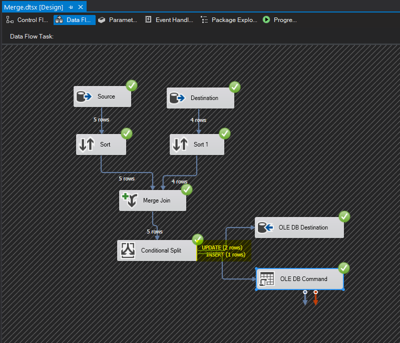
Cross fingers and hit Execute.

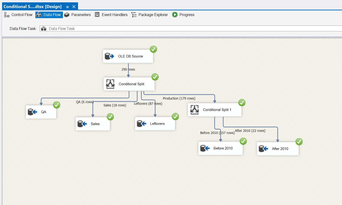
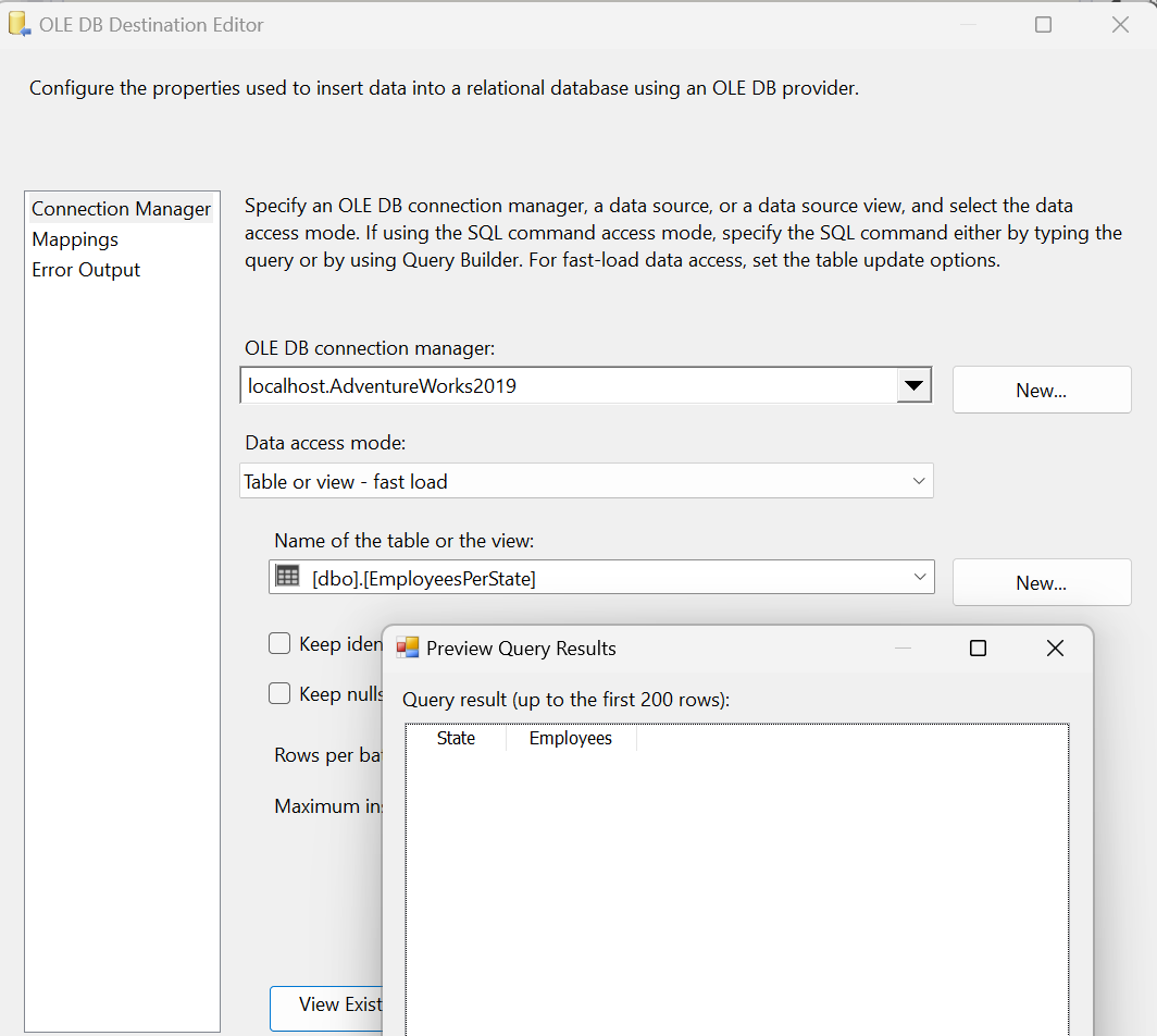
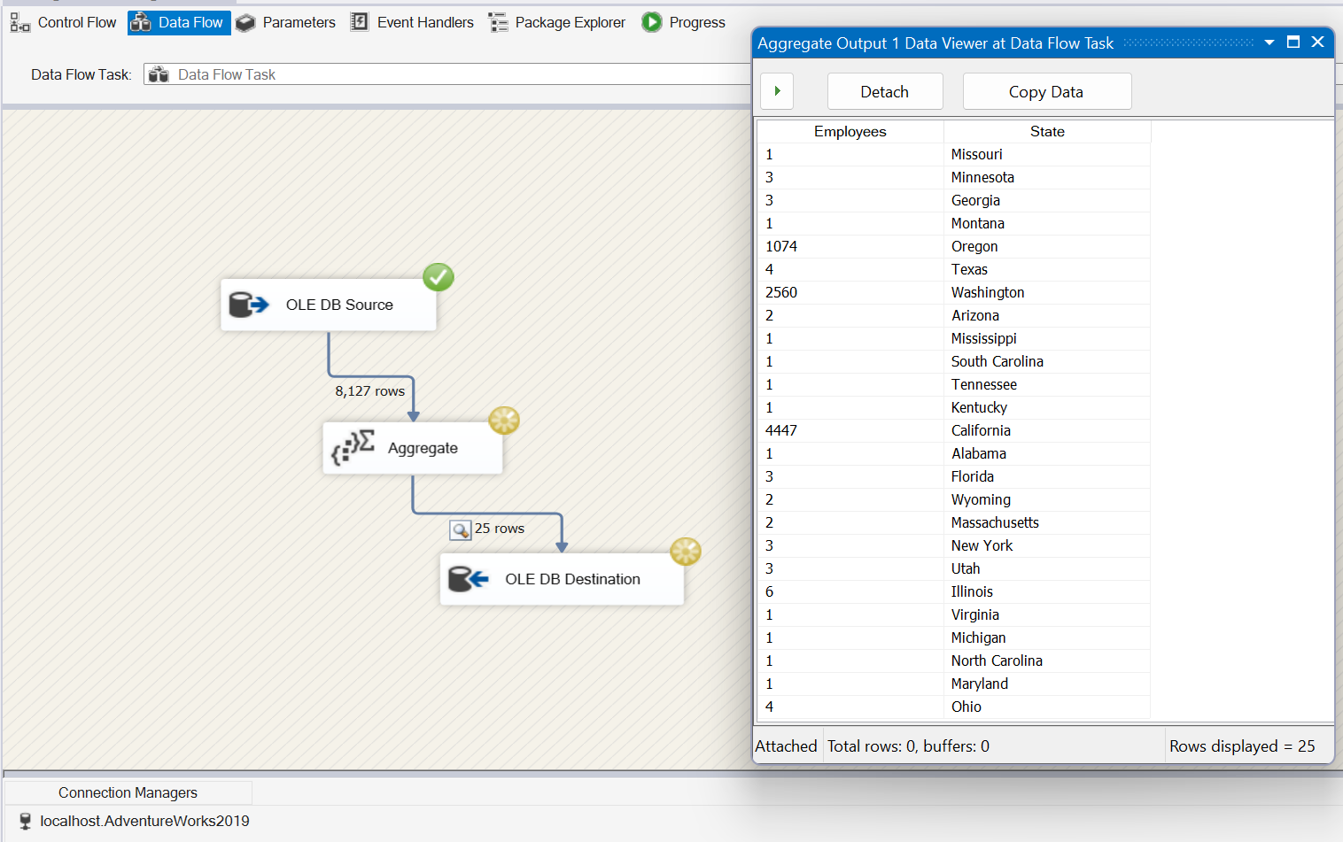
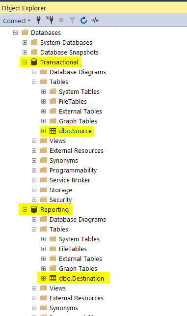
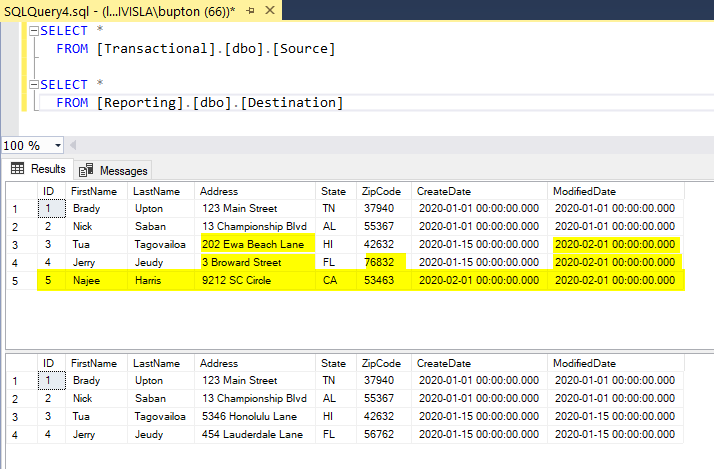
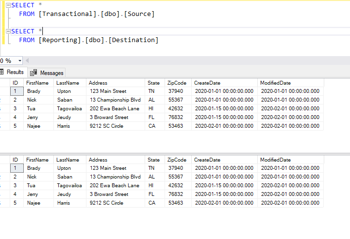
Yay, no red X! Let’s take a look at our SQL tables to make sure everything exported correctly.

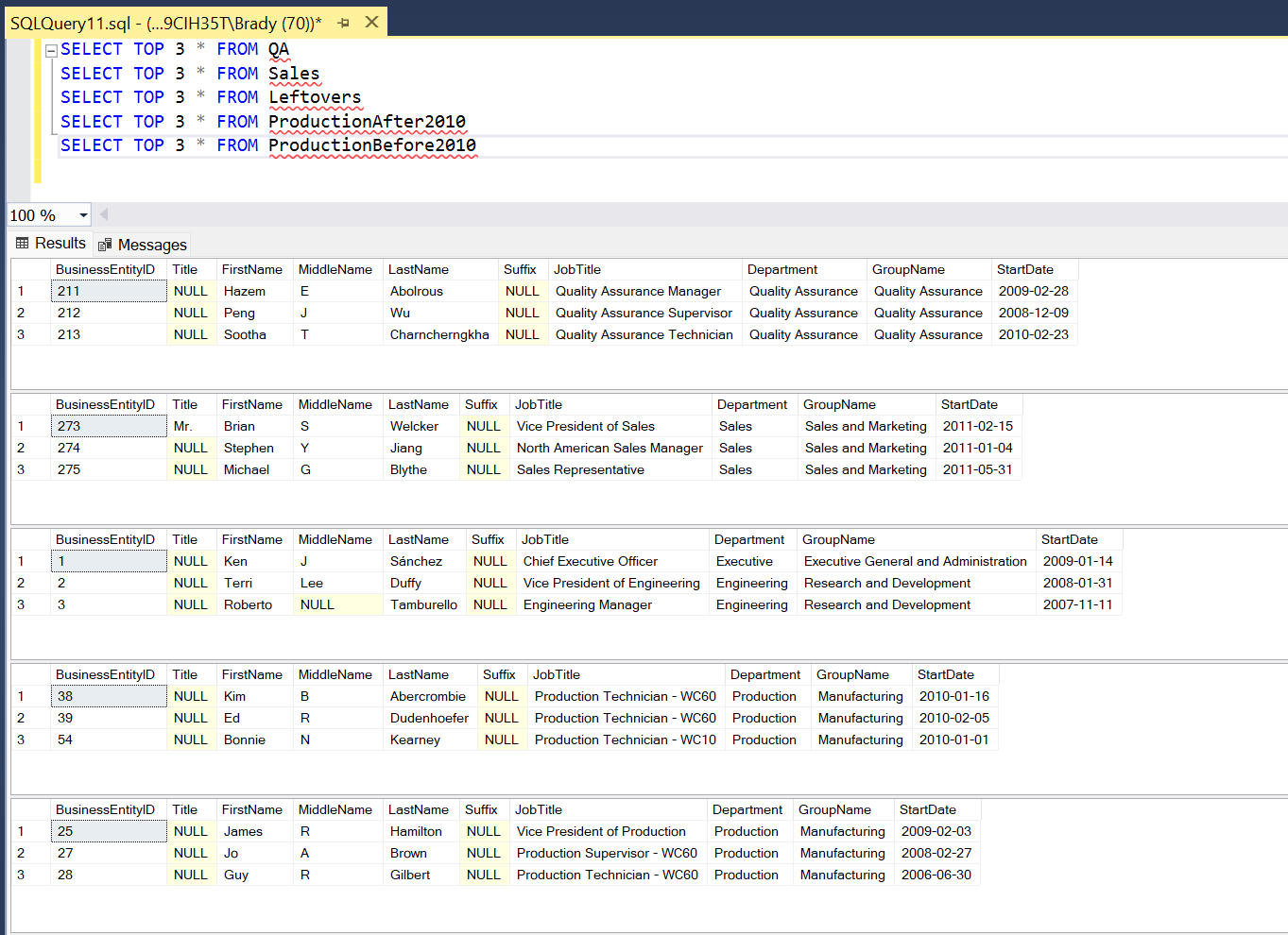
Boom. Let’s go grab a bourbon!

SSIS Series: How to use SSIS Balanced Data Distributor

By bradyupton in Business Intelligence, Integration Services (SSIS), SSIS Series January 14, 2023 0 Comment

From Microsoft, the Balanced Data Distributor (BDD) transformation takes advantage of concurrent processing capability of modern CPUs. It distributes buffers of incoming rows uniformly across outputs on separate threads. By using separate threads for each output path, the BDD component improves the performance of an SSIS package on multi-core or multi-processor machines.

The Balanced Data Distributor transformation helps improve performance of a package in a scenario that satisfies the following conditions:

There is large amount of data coming into the BDD transformation. If the data size is small and only one buffer can hold the data, there is no point in using the BDD transformation. If the data size is large and several buffers are required to hold the data, BDD can efficiently process buffers of data in parallel by using separate threads.
The data can be read faster than the rest of the data flow can process it. In this scenario, the transformations that are performed on the data run slowly compared to the rate at which data is coming. If the bottleneck is at the destination, the destination must be parallelizable though.
The data does not need to be ordered. For example, if the data needs to stay sorted, you should not split the data using the BDD transformation.

Let’s dive in and take a quick look at how the Balanced Data Distributor works.

Go ahead and open Visual Studio, it might take a minute to load.

We’re going to use AdventureWorks2019 database for this example. The SalesOrderDetail table has over 121k records so that’s a good candidate.

SELECT * FROM Sales.SalesOrderDetail

Now that we have data let’s go back over to Visual Studio and see if it’s still spinning.

Drag in a Data Flow task, double click to open and then let’s drag in an OLE DB Source and a Flat File Destination task.

I’m going to configure the source to point to my AdventureWorks2019 database and the destination to point to a .csv file on my local laptop.

Easy enough. Let’s go ahead and run this and see what happens.

We can see that our 121k rows were written to our CSV file and the CSV file ended up being 12.3 MB. That’s pretty large for an email file attachment and might crash your laptop even trying to open this file. BDD not only offers performance benefits by using multiple threads, but it can also break up large files into smaller ones. IMO, this is what makes this task great.

We need to get this file down to less than 4MB so we’ll need to break this up 4 times. With that said, let’s add the BDD task between the source and destination tasks. There is nothing configurable *in* this task, however, there are some properties that may need to be tweaked. After adding the BDD task, we’ll need to add 3 more flat file destination tasks and 3 more flat file connection managers. End result should look something like this:

That’s really about it. Let’s fire it off and see the results of our flat files.

It worked! 121k rows were written across 4 flat files. Our flat file size is less than 4MB each and we can send these very easily via email. This is a very quick and easy way to split data between files, however, there is no order to these records so an ORDER BY is not helpful here. If the goal is to separate data by a category or condition then you’ll need to use a Conditional Split task which I wrote about in this post.

SSIS Series: How to use SSIS Aggregate Data Flow Task – Basic and Advanced

By bradyupton in Business Intelligence, Integration Services (SSIS), SSIS Series January 7, 2023 0 Comment

From Microsoft, the Aggregate transformation applies aggregate functions, such as Average, to column values and copies the results to the transformation output. Besides aggregate functions, the transformation provides the GROUP BY clause, which you can use to specify groups to aggregate across.

The Aggregate transformation supports the following operations.

Operation	Description
Group by	Divides datasets into groups. Columns of any data type can be used for grouping. For more information, see GROUP BY (Transact-SQL).
Sum	Sums the values in a column. Only columns with numeric data types can be summed. For more information, see SUM (Transact-SQL).
Average	Returns the average of the column values in a column. Only columns with numeric data types can be averaged. For more information, see AVG (Transact-SQL).
Count	Returns the number of items in a group. For more information, see COUNT (Transact-SQL).
Count distinct	Returns the number of unique nonnull values in a group.
Minimum	Returns the minimum value in a group. For more information, see MIN (Transact-SQL). In contrast to the Transact-SQL MIN function, this operation can be used only with numeric, date, and time data types.
Maximum	Returns the maximum value in a group. For more information, see MAX (Transact-SQL). In contrast to the Transact-SQL MAX function, this operation can be used only with numeric, date, and time data types.

This transformation could also be implemented with a SQL query after an initial load, but this task makes it nice to take care of the transformation within SSIS so that the data is ready on export. Let’s take a quick look at how it works.

Using AdventureWorks database, I’ll run the following query which gives me everyone in the Person.Person table that is located in the US.

SELECT firstname + ' ' + lastname AS PersonName, AddressLine1, AddressLine2, City ,sp.[Name] AS STATE, PostalCode, CountryRegionCode FROM person.Person p JOIN person.BusinessEntityAddress bea ON p.BusinessEntityID = bea.BusinessEntityID JOIN person.Address a ON bea.AddressID = a.AddressID JOIN person.StateProvince sp ON a.StateProvinceID = sp.StateProvinceID WHERE CountryRegionCode = 'US'

For this post, let’s pretend our boss wants to see how many people we have in each state. So a simple COUNT(*) and GROUP BY State query would work, but we’ll use SSIS to export this into a table using the Aggregate task.

Fire up Visual Studio and let’s create a Data Flow Task, add source connection and destination connection.

Next, let’s add our Aggregate task between our Source and Destination and open the editor:

This example is pretty straightforward as we want to do a COUNT on all records so we’ll choose (*) under Input Column, give it a name under Output Alias and the only available option for * is Count All.

Next, we want to get the number of people per state, so we’ll add State to our Input Column, give it a name, and select GROUP BY for our operation:

We can use multiple options on this screen such as SUM, AVG, MIN, MAX, etc. depending on data types.

Hit OK on the screen which will take us back to our Data Flow task. Taking a look at our Destination task, you can see I have a table named EmployeesPerState with only two columns, Employee and State:

Save the package and execute and you can see that we’ve inserted the data we need. Boss is happy and gives you a $6 bonus.

For Advanced Mode, you can create more than 1 GROUP BY criteria. For example, the boss now wants to see the number of people in each state, but he also wants to see how many people per zip code. For this, we would expand the Advanced/Basic drill down and add another input for his request. We’ll name the Aggregation PostalCode and Group by PostalCode. Like we did for our State aggregation, we’ll add a Count all Operation and (*) Input.

Back on the Data Flow task, we’ll drag another Destination task into the editor and configure.

You can now see both Destination tasks with a label for each.

If we run the package again, you can see results have been inserted into our PostalCode table and the boss gives you another $6 bonus and let’s you take Sunday off.

SSIS Series: Insert/Update a SQL Server table using Merge Join in SSIS

By bradyupton in Business Intelligence, Integration Services (SSIS), SSIS Series April 25, 2020 0 Comment

I was asked a question awhile back on the easiest way to do an incremental load from one SQL Server table into another SQL Server table. This is common in data warehouses or reporting tables as you wouldn’t want to truncate a large table and perform a full insert. Instead, you would want to only copy the changes from the source to the destination. This could be an insert or an update. The easiest way, IMO, is SSIS. Let’s take a look.

Here’s how my environment is setup. I have two databases appropriately named Transactional (for transactional data) and Reporting (for static report data). Two tables, Source and Destination.

I also added some dummy data as you see below. I’ve highlighted what is different and will need to be changed in the destination table.

Let’s open SSIS and create a new SSIS project.
Drag and drop a Data Flow task into the design window, right click, Edit:

Next, drag and drop two OLE DB source components into the design window. I’m going to rename mine Source and Destination to match my table names.

Configure the two OLE DB sources to match the source table and the destination table. Below is a screenshot of my source connection manager.

Once your connection managers are configured let’s drag and drop two Sort components below each OLE DB Source and connect them to each source. We will be using a merge join next and the merge join component needs to have data sorted in ASC or DESC order. I always choose to sort on the Primary Key for each table.

In my example, I’ll choose to sort on my primary key, ID.

Next, drag the Merge Join transformation into the Design window and drag the data path from the Sort component to the Merge Join. When you attach the arrow to the transformation, the Input Output Selection dialog box appears, displaying two options: the Output drop-down list and the Input drop-down list. The Output drop-down list defaults to Source Output, which is what we want. From the Input drop-down list, select Merge Join Left Input, as shown below. We’ll use the other option, Merge Join Right Input, for the other connection.

Next, connect the data path from the other Sort component to the Merge Join transformation. This time, the Input Output Selection dialog box does not appear. Instead, the Input drop-down list defaults to the only remaining option: Merge Join Right Input.

Now, let’s configure the Merge Join transformation.

The first setting in the Merge Join Transformation Editor is the Join type drop-down list. From this list, you can select one of the following three join types:

Left outer join: Includes all rows from the left table, but only matching rows from the right table. You can use the Swap Inputs option to switch data source, effectively creating a right outer join.
Full outer join: Includes all rows from both tables.
Inner join: Includes rows only when the data matches between the two tables.

For our example, we want to include all rows from left table but only rows from the right table if there’s a match, so we’ll use the Left outer join option.

You now need to select which columns you want to include in the data set that will be outputted by the Merge Join transformation. For this exercise, we’ll include all columns. To include a column in the final result set, simply select the check box next to the column name in either data source.

Almost finished, but first let’s add a Conditional Split transformation. This will allow us to insert new records or update previous records.

In the Conditional Split Editor, I created two outputs. If (Destination) ID is NULL then the record doesn’t exist so we’ll perform an INSERT. If the ModifiedDate is different between the two tables then we know something has been updated since the last execution and we need to update the record. See below.

Since we can perform and INSERT or an UPDATE we’ll need two destinations. First, for the INSERT, we’ll simply be doing an INSERT into the table so we can drag the OLE DB Destination component into the window, choose “INSERT” in the Input Output selection window, and use the Reporting connection manager.

I’m going to check the “Keep Identity” box since the ID column is an identity column.

Next, for the UPDATE statement we’ll drag the OLE Command component into the window and configure it. Select “UPDATE” in the Input Output Selection window.

In the Connection Managers tab, assign the connection manager for Reporting.

In the Connection Managers tab, assign the connection manager for Reporting.

In the column mappings tab, assign parameters:

Final package should look like the following:

Save and execute. You can see that we updated two records and inserted one record:

Going back to our query you can see that everything matches up now:

Using Bookmarks in Power BI

By bradyupton in Business Intelligence, Development, Power BI March 13, 2019 0 Comment

Using bookmarks in Power BI help you capture the currently configured view of a report page, including filtering and the state of visuals, and later let you go back to that state by simply selecting the saved bookmark.

You can also create a collection of bookmarks, arrange them in the order you want, and subsequently step through each bookmark in a presentation to highlight a series of insights, or the story you want to tell with your visuals and reports.

In this post we’ll quickly go over how to create a few bookmarks and view them as a slideshow if you will.

I’m going to use my March Madness Report I created in an earlier post. Once my report is opened in Power BI Desktop, I’m going to click on the View tab in the ribbon and select “Bookmarks Pane”

This should bring up a new Bookmarks pane inside PBI Desktop:

Remember, bookmarks are used to capture the current view of the report so I’m going to use the default view where I’m showing all data and I’m going to name the bookmark “Home”. Make sure all filters are selected to show all data and click Add under the bookmark pane. This will create a new Bookmark, named Bookmark 1. Click the ellipsis and select rename to rename the bookmark appropriately.

Next, I like North Carolina, so I’m going to go to my Team Filter and choose North Carolina which will show me data for only this team.

In my bookmark pane, I’m going to click Add again and rename to North Carolina.

Next, I want to view data on North Carolina from 2000 to present so I’ll change the Year Filter.

In my bookmark pane, I’m going to click Add again and rename to North Carolina 2000-present.

Now, if I click on any of bookmarks, it will take me to the data that was saved for each. This is a great way to present data in a meeting/conference so you don’t have to manually change the filters during the engagement.

We can also click the View button in the Bookmark pane to view a slideshow using the arrows at the bottom to navigate:

Creating a Dynamic Date Range Title in Power BI

By bradyupton in Business Intelligence, Development, Power BI March 5, 2019 0 Comment

Creating a dynamic title in Power BI helps present the data and let’s the viewers know what the data is filtered on. In this post I’ll go over how to do this…

I have a sales report that I’d like to add a title that is based on the Order Date Slicer. Currently, the title is static text “Sales Report”

To create my dynamic title, I’ll first need to create a measure table that has my Order Date data. In this case, that table is FactInternetSales and the column is OrderDate.

To create a measure, click New Measure in the Power BI Desktop ribbon

Next, you’ll see a window where you can type code. In this example, I’ll use the following DAX

Order Date Title = “Sales For ” &
MIN ( FactInternetSales[OrderDate] ) & ” to “
& MAX ( FactInternetSales[OrderDate] )

Let’s walk through this real quick.

The first line (Order Date Title = “Sales For “ &) is basically naming the measure and adding the beginning text for the title.
The second line (MIN ( FactInternetSales[OrderDate] ) & “ to “) is finding the minimum order date from FactInternetSales.OrderDate and then adding the “to” text.
The last line (MAX ( FactInternetSales[OrderDate] ) is finding the maximum order date from FactInternetSales.OrderDate.

This one was pretty easy. Once I’ve typed my DAX, hit the checkmark to make sure there are no errors and the click off screen.

Our measure has been created! Let’s go back and find it under the FactInternetSales fields pane.

Next, let’s click on the Card Visualization and move and size it appropriately to fit in our title space.

While the card is highlighted, click on the new measure from the Fields pane and it will populate the card with the measure we created.

The only thing left to do is format the title and we’re all set! If we change the Order Date Slicer, you’ll notice the title changes with the date. See live example at the beginning of this post.

March Madness Power BI Dashboard

By bradyupton in Business Intelligence, Development, Power BI February 21, 2019 0 Comment

At the beginning of the year I set a goal to learn something new. I’ve always loved business intelligence and bringing data to life in the form of dashboards and charts so for the 1^st half of the year I wanted to focus on Microsoft’s Power BI. I’m not going to explain what Power BI is, but if you want to read up on it go here: https://powerbi.microsoft.com/en-us/

This post is just going to show off my dashboard. ? See live example above.

I’m a huge sports fan and the best time of the year happens to fall in March. Besides my birthday being in March, it’s also March Madness. Hours and hours of basketball. I could of used AdventureWorks for my dataset, but I wanted to use something I’m interested in. I found some data containing every NCAA tournament game result since 1985 (when the tournament was expanded to the 64 team bracket). The dataset contains the year, round (1-6), seed of the teams (1-16), region (1-4) and the scores. Perfect. Let’s use this to create a dashboard.

There’s not a ton of data, but I used what I could and tried to answer some questions around wins and upsets. Here’s a screenshot of the final product:

You can see Wins By Team (Duke with 93, North Carolina with 78, etc), Wins by Seed, National Championships, and Upsets vs Wins by Year. You can also see that a total of 2142 games have been played with 199 different teams in the tournament.

This was really fun and answers a lot of the questions I was thinking in my head while designing. The top left corner also has slicers which help filter the data. For example, if I wanted to see only the data for 2015 I could change the Year slicer to 2015 and it would update all my visualizations:

March Madness Power BI Dashboard filtered by year 2015

You can see that Duke won the National Championship from the National Championships visualization. If you hover over the Wins and Upsets visualization, you’ll see there were 30 upsets out of 63 games.

Let’s say I want to view data for a certain Team. Let’s choose Alabama Crimson Tide. If I change the Team slicer to Alabama I can see some data based around this team.

March Madness Power BI Dashboard filtered by team Alabama Crimson Tide

Alabama has won 19 NCAA tournament games, 0 national championships, has been a 5 or 7 seed 21% of the time and they’ve had a few upsets along the way. Not bad for a football school.

What about data for the National Championship game? I can change the Round slicer to 6, which is the National Championship round and view the data this way.

March Madness Power BI Dashboard filtered by Championship game

I can see out of 34 games, there has only been 16 different teams make the National Championship. Duke leads the way with 6, followed by North Carolina and Connecticut with 4. The 1 seed has played in this game 59% of the time, and there were upsets in 1988, 1990, 1997, 2003, 2006, and 2016.

We can also click on the visualizations themselves to view data. For example, if we reset our slicers to show all data and click on the #1 seed in the Wins By Seed Donut Chart we see the following:

March Madness Power BI Dashboard filtered by #1 seed

We can see that the #1 seed has played in 419 games with a total of 41 different teams. Duke has won 51 games as the #1 seed while North Carolina has won 46. Duke has also won the National Championship 4 times as the #1 seed and in 1999 the #1 seed won 17 games which is the highest.

Really cool stuff. I loved working on this project and working with this data.

Using a DateTime Expression in a SSIS Destination

By bradyupton in Business Intelligence, Integration Services (SSIS) April 17, 2015 0 Comment

Recently, I’ve ran into a few situations where I needed to export some SQL data into a CSV on a daily basis. I also needed to keep these CSV files in an archive folder for reference in case a problem came up. Moving the files to an archive folder is not a problem using the “File System” task, but the CSV needs to be a unique name otherwise it will just overwrite the previous file. There are numerous ways to make the filename unique, but in the post I’ll describe adding a datetime stamp to each file which also helps determine when the file was created.

I’ll assume you already have a Data Flow task configured with a destination and a flat file source. In this example, I’m going to use the AdventureWorksDW2012 database and copy data from the DimProduct table to a CSV. I already have my OLE DB source task configured and now I’m going to configure the Flat Destination.

Right click the Flat File Destination and click Edit:

In the Flat File Destination Editor, click New…

Select Delimited and click OK.

I’ve created a blank CSV on my Desktop which we’ll use for now, but this will eventually change:

Click OK and select Mappings and verify all the mappings from the source are correct:

Once this is verified, click OK. (For this example, I only want to copy the first 6 columns)

Next, we need to create an expression on the connection string so that it knows to add the datetime stamp. Click on the Flat File Connection Manager. Scroll down the Properties window until you see Expressions:

Click the ellipsis beside Expressions and the Property Expressions Editor will appear:

Under Property, select Connection String and click the ellipsis under Expression:

You should now see the Expression Builder window. Here is where we will define our complete file name including file path. For this example, I want to create the CSV in a directory named CSV on the C: drive. The filename that I will use is Products_datetime stamp.csv so the final output should be C:\CSV\Products_20150417092331.csv

The expression I’ll use to achieve this is below:

"C:\\CSV\\Products_" + (DT_STR,4,1252)DATEPART( "yyyy" , getdate() ) + RIGHT("0" + (DT_STR,4,1252)DATEPART( "mm" , getdate() ), 2) + RIGHT("0" + (DT_STR,4,1252)DATEPART( "dd" , getdate() ), 2) + RIGHT("0" + (DT_STR,4,1252)DATEPART( "hh" , getdate() ), 2) + RIGHT("0" + (DT_STR,4,1252)DATEPART( "mi" , getdate() ), 2) + RIGHT("0" + (DT_STR,4,1252)DATEPART( "ss" , getdate() ), 2) + ".csv"

Type your expression in the Expression window of the Expression builder:

Click Evaluate Expression to view the output:

Now that the expression is built, click OK twice. You should now see the expression formula icon beside the Flat File Connection Manager:

If we execute the package and look inside the CSV folder, you should see our new file:

SQL Server Integration Services Connector for SalesForce

By bradyupton in Business Intelligence, Integration Services (SSIS) February 26, 2015 1 Comment

Problem:

I have a list of contacts in my SQL Server database that I would like to import into Salesforce and keep Salesforce up to date as new contacts are entered daily into my database. I know there are a few different ways to accomplish this but I’d like to use a SSIS package so I can automate.

Solution:

In my opinion, the best (and easiest) way to accomplish this goal is using SSIS packages and a component from CozyRoc called Salesforce Destination. CozyRoc provides advanced SSIS libraries of custom tasks, components and scripts for handling Zip, GZip, BZip2, Tar archives, enhanced script reuse and secure Internet communications. I always go to CozyRoc when I need a custom task. In this tip I’ll show you how to take a contact list from SQL Server and import it into SalesForce. I’ll also show you how to schedule this on a daily basis.

For this example, let’s say I have a contact table in my SQL Server database like the following:

I need to import these records into my Contacts tab in SalesForce:

Create SSIS package

First thing I’ll need to do is download the CozyRoc SalesForce component. This download can be found here: http://www.cozyroc.com/ssis/salesforce-destination

I’ll download and install this component on the server or workstation that I plan on developing the package. Once installed, open SQL Server Data Tools and create a SSIS project:

First, let’s create a connection to the SQL Server database that stores the contact information and the Salesforce destination:

Right click in Connection Manager and create “New OLE DB Connection”:

Type Server Name, credentials, and select database from drop down that stores the contact information. In this example, I’m selecting my local server and Demo database:

Test Connection and click OK. Right click on the Connection Manager again and click “New Connection”:

If the Salesforce Destination component was installed properly, you should see a connection called “SFORCE”:

Click Add. Type your UserName and Password + Security token. If you don’t know your security token click here to read more about resetting it.

Once you have entered your login credentials, make sure to test connection.

You should now have two connections in Connection Managers:

Now to designing the package:

From the Control Flow we will add our Data Flow Task and right click to configure.

Add the OLE DB source and SalesForce Destination tasks to the designer:

Configure OLE DB Source:

To configure the SalesForce Destination right click and edit. Choose the connection manager you created earlier:

Click the Component Properties tab and you’ll notice a few options under Custom Properties:

Action:

Action	Description
Create	Create a new record in the destination object
Update	Update an existing record in the destination object. You must specify the appropriate object record identifier for the update to work.
Delete	Delete an existing record from the destination object. You must specify the appropriate object record identifier for the delete to work.
Upsert	Update and insert a record in the destination object. Selecting this value displays the dynamic parameter ExternalId.

Batch Size: Specify the number of rows to be sent as a batch. The maximum for regular mode is 200. The maximum for bulk-load is 10,000\.

Destination Object: Specify the destination Salesforce object from a dropdown where the data is to be loaded.

ExternalID: Specify the external identifier field for updating the foreign key lookup with an external identifier.

Mode:

Value	Description
Regular	Process the data in regular mode
BulkData	Process the data in bulk-load data mode
BulkBinary	Process the data in bulk-load binary mode

Since we are adding Contacts, we’ll select Create (Action) and Contact from the DestinationObject option.

Click the Column Mappings tab and make sure all the columns are mapped correctly (delete mapping between ID’s for this example):

Run the package and if everything is setup correctly your Salesforce instance should new contacts in it:

Run this package as daily job

To run this package as a daily job that will populate Salesforce hourly, daily, weekly, etc. we’ll need to create a SQL Agent job and set a schedule.

Next Steps:

Updating Salesforce is a little more complicated and requires a custom field in Salesforce. The video titled “Upsert with external ID” located here will help with this.
Check out com for your custom SSIS needs.

Collect SQL Server Performance Counters and Build Reports with SSRS

By bradyupton in Business Intelligence, Monitoring, Reporting Services (SSRS) February 26, 2014 1 Comment

Third party tools are awesome for capturing performance metrics, but some small shops (and even large shops) don’t budget for this type of software leaving it up to the DBA to create their own monitoring solution.

There are a few different ways to capture certain performance metrics, but in this post I’ll focus on using the sys.dm_os_performance_counters DMV and how to view this data in a more readable form using SQL Server Reporting Services graphs. The DMV doesn’t include all the counters as Performance Monitor, but it does show the SQL Server related counters. (Note that some of the counters in this DMV are of cumulative values since the last reboot.)

You can query this DMV using the following query:

SELECT * FROM sys.dm_os_performance_counters

SQL Freelancer SQL Server Performance Counters SSRS

As you can see from the screenshot above, this can be hard to read. Also, it only shows the current values at the time the query is executed so you don’t know anything about the past and it makes it hard to see how the data fluctuates during the business day.

Collecting the SQL Server Monitoring Report Data

For the purpose of simplicity, this tip will focus on one counter, Page Life Expectancy (PLE). I’ll show you how to capture data and create a graph for analysis.

First, we’ll need to create a table that will store our metrics:

CREATE TABLE [dbo].[CounterCollections](
[ID] [int] IDENTITY(1,1) NOT NULL,
[object_name] [varchar](128) NOT NULL,
[counter_name] [varchar](128) NOT NULL,
[cntr_value] [bigint] NOT NULL,
[collection_datetime] [datetime] NOT NULL )

Next, we’ll need to create a script that will insert our data into the table we created above:

INSERT INTO CounterCollections
SELECT object_name, counter_name, cntr_value, GETDATE() collection_datetime
FROM sys.dm_os_performance_counters
WHERE object_name = ‘SQLServer:Buffer Manager’
AND counter_name = ‘Page life expectancy’

Finally, we’ll need to create a SQL Server Agent Job that will run the script above on a specified schedule:

I’ll run this job every 5 minutes:

Creating the SQL Server Monitoring Report

While the table gathers data we can switch over to Business Intelligence Development Studio (BIDS) or the SQL Server Data Tools (SSDT) and create a SSRS Report that will display our data.

In this example, I’m using SSDT. Choose File, New Project. On the New Project dialog choose Report Server Project and name the Project:

Click here to view the rest of this post.