Now that SQL Server 2019 has finally been released click the link below to view the new features.
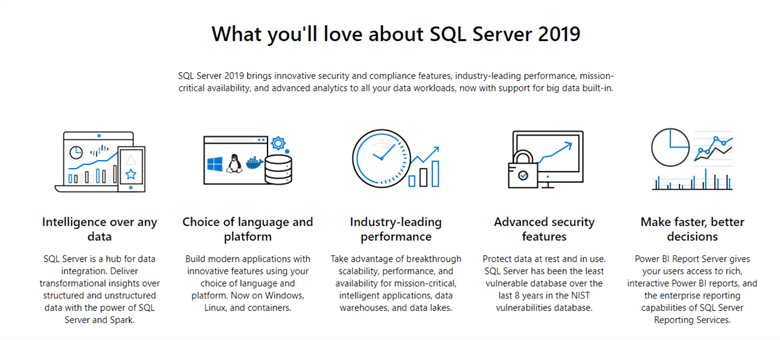
https://docs.microsoft.com/en-us/sql/sql-server/what-s-new-in-sql-server-ver15?view=sql-server-ver15
Now that SQL Server 2019 has finally been released click the link below to view the new features.
https://docs.microsoft.com/en-us/sql/sql-server/what-s-new-in-sql-server-ver15?view=sql-server-ver15
Support for SQL Server 2008 and 2008 R2 ended on July 9, 2019. That means the end of regular security updates. However, if you move those SQL Server instances to Azure or Azure Stack, Microsoft will give you three years of extended security updates at no additional cost. If you’re currently running SQL Server 2008 or 2008 R2 and you are unable to update to a later version of SQL Server, you will want to take advantage of this offer rather than running the risk of facing a future security vulnerability. An unpatched instance of SQL Server could lead to data loss, downtime, or a devastating data breach.
If you have a SQL Server failover cluster instance (FCI) or use hypervisor-based high availability, or other clustering technology on-premises for high availability, you’ll probably need the same in Azure. If you need to migrate to Azure/Azure Stack at end of support, and you require high availability for SQL Server 2008/2008 R2, there’s only one solution recommended by Microsoft: SIOS DataKeeper. SIOS DataKeeper enables clustering in the cloud, including the creation of a SQL Server 2008/2008 R2 failover cluster instance, allowing you to achieve your high availability goals.
Planning and building SQL Server in RDS doesn’t have to scare you. It’s actually pretty easy and in this post will go over planning a SQL Server deployment in RDS, creating SQL Server in RDS, and last but not least configuring the new instance of SQL Server.
Let’s jump in…
Planning the deployment is important because if your SQL Server instance needs a feature that RDS doesn’t support, then RDS isn’t an option. Here are a few, but you can get the full list here: https://docs.aws.amazon.com/AmazonRDS/latest/UserGuide/CHAP_SQLServer.html
RDS also has some limitations that don’t exist with an on-premise SQL Server. Let’s look at a few:
Again, the full list can be found here: https://docs.aws.amazon.com/AmazonRDS/latest/UserGuide/CHAP_SQLServer.html
Pricing
Once you can verify that your environment will run properly in RDS you’ll need to look at the pricing model. When you setup RDS for SQL Server, the software license is included. AWS used to have a program called “Bring your own license” or “BYOL”, which allowed you to use a license that was already bought from Microsoft via an agreement or other. This has been rumored to expire on June 30, 2019. The software license that is included means that you don’t need to purchase SQL Server licenses separately. AWS holds the license for the SQL Server database software. Amazon RDS pricing includes the software license, underlying hardware resources, and Amazon RDS management capabilities. The pricing will depend on the selections such as size, edition, etc.
The following editions are supported in RDS:
Notice, Developer Edition is not included with RDS and Web Edition supports only public and internet-accessible webpages, websites, web applications, and web services.
Instance Type
You can also choose from On-demand or reserved instances. On-Demand DB Instances let you pay for compute capacity by the hour your DB Instance runs with no long-term commitments. This frees you from the costs and complexities of planning, purchasing, and maintaining hardware and transforms what are commonly large fixed costs into much smaller variable costs. This is good for development environments where you can power on and off the server as it’s being used.
Reserved Instances give you the option to reserve a DB instance for a one or three year term and in turn receive a significant discount compared to the On-Demand Instance pricing for the DB instance. Amazon RDS provides three RI payment options — No Upfront, Partial Upfront, All Upfront — that enable you to balance the amount you pay upfront with your effective hourly price.
You can see more about on-demand vs reserved instances and pricing here: https://aws.amazon.com/rds/sqlserver/pricing/
RDS provides a selection of instance types optimized to fit different relational database use cases. Instance types comprise varying combinations of CPU, memory, storage, and networking capacity and give you the flexibility to choose the appropriate mix of resources for your database. Each instance type includes several instance sizes, allowing you to scale your database to the requirements of your target workload. View more details here: https://aws.amazon.com/rds/instance-types/
Storage
Another item to look at when planning your deployment is storage. RDS uses Amazon Elastic Block Store (Amazon EBS) volumes for database and log storage. Depending on the amount of storage requested, Amazon RDS automatically stripes across multiple Amazon EBS volumes to enhance performance.
RDS offers three different storage types:
General Purpose SSD – also called gp2, this storage type offers cost-effective storage that can be used for a broad range of different workloads. These volumes deliver single-digit millisecond latencies and the ability to burst to 3,000 IOPS for extended periods of time. I would recommend putting small to medium sized databases on this type.
Provisioned IOPS – This storage type is designed for I/O intensive workloads, particularly database workloads that require low I/O latency and consistent throughput. This is also built on SSD and targeted for IO intensive, high performance databases. Cost wise, this is the highest of the three storage types.
Magnetic – This storage type is mostly used for backward compatibility. Amazon recommends using gp2 or Provisioned IOPS for any new builds. This is ideal for test and dev environments when performance isn’t a concern. This is the cheapest of the three storage types.
See more about storage here: https://docs.aws.amazon.com/AmazonRDS/latest/UserGuide/CHAP_Storage.html
Network
One more item to consider when planning the deployment is network connectivity. Applications will more than likely need to connect to your RDS environment so there are a few import concepts to look at it.
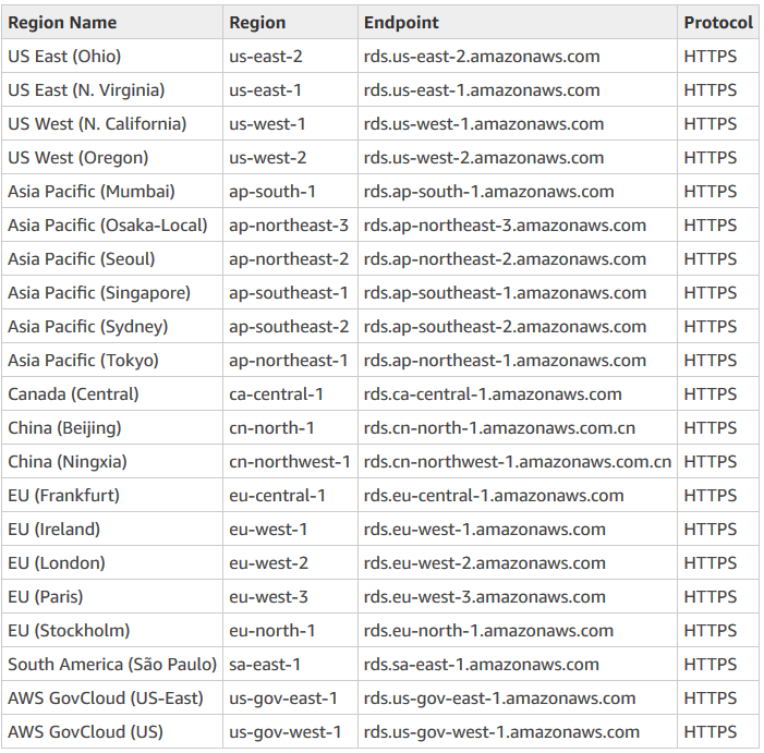
Availability Zones – this is simply a data center in an AWS region. The following AWS regions exist.
Virtual Private Cloud – also called VPC, this is an isolated virtual network that can span multiple Availability Zones. It’s used to group different types of resources to the network that need to talk to each other.
Virtual Private Cloud – also called VPC, this is an isolated virtual network that can span multiple Availability Zones. It’s used to group different types of resources to the network that need to talk to each other.
DB Subnet Group – this is a collection of subnets inside a VPC that contains the RDS instance addresses. See more about VPC and DB subnet groups here: https://docs.aws.amazon.com/AmazonRDS/latest/UserGuide/USER_VPC.WorkingWithRDSInstanceinaVPC.html
Create SQL Server RDS via AWS Console
Now that we’ve outlined some of the deployment planning tasks, let’s build an instance through the AWS console.
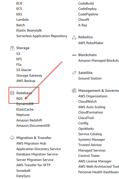
Once inside the console, we’ll click on RDS under the Database heading:
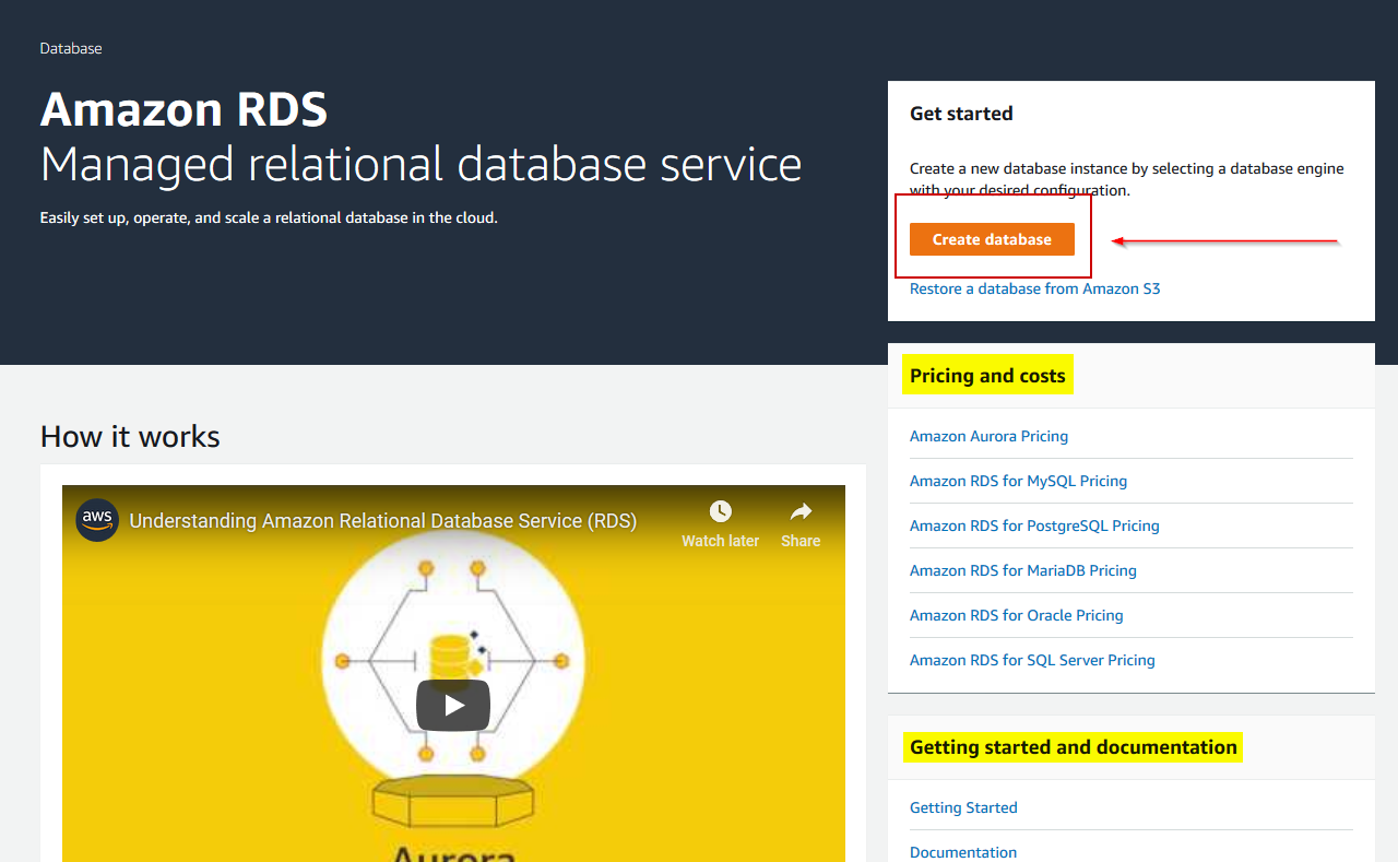
Once we are on the home page for RDS, we can click Create Database under Get Started. There’s also info for Pricing and costs and some documentation on getting started:
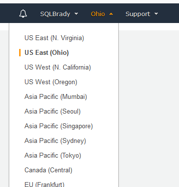
Notice in the top right corner is the Availability Zone in which you are logged into. In my case, I’m logged into US East (Ohio) since I’m on the Central Time Zone and Ohio is located closer to me than any other zone:
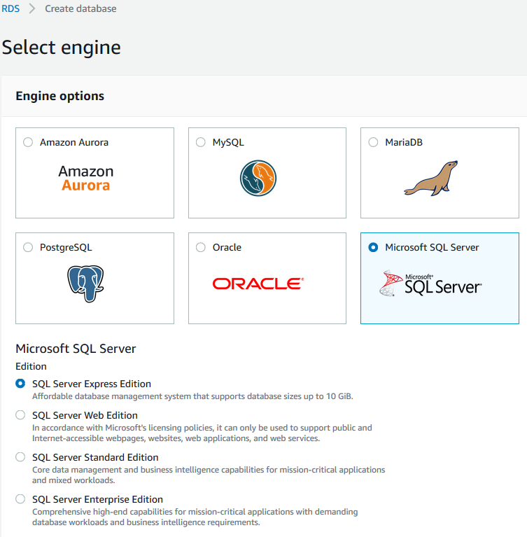
Back to the Select Engine page. For this post, I’m going to install Microsoft SQL Server Express, but you can see the other database engine platforms that are available and the associated editions:
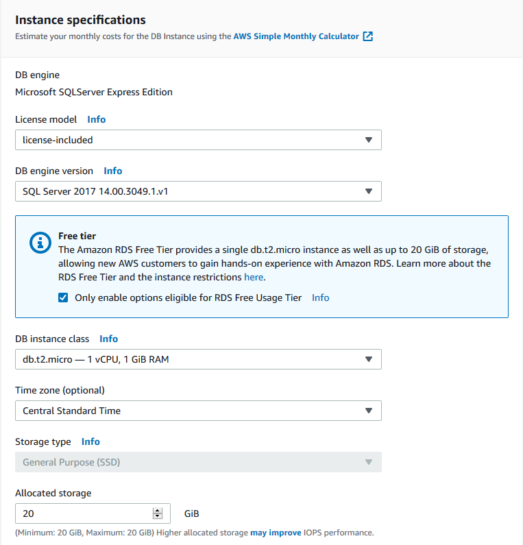
Next page we can see some of our database details. There are all items we discussed in the planning deployment section above. License model, DB engine version, DB instance class, Time Zone, Storage Type and allocated storage are all configurable on this page. Below are my selections:
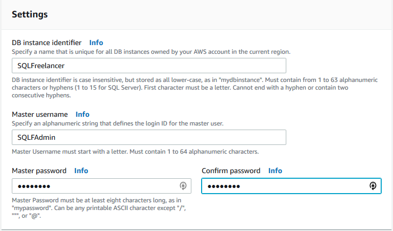
Scroll down to Settings header and configure the DB instance identifier, Master username and password. The DB instance identifier is a unique name for your DB instances across the current region. For this RDS instance I’ll name it SQLFreelancer:
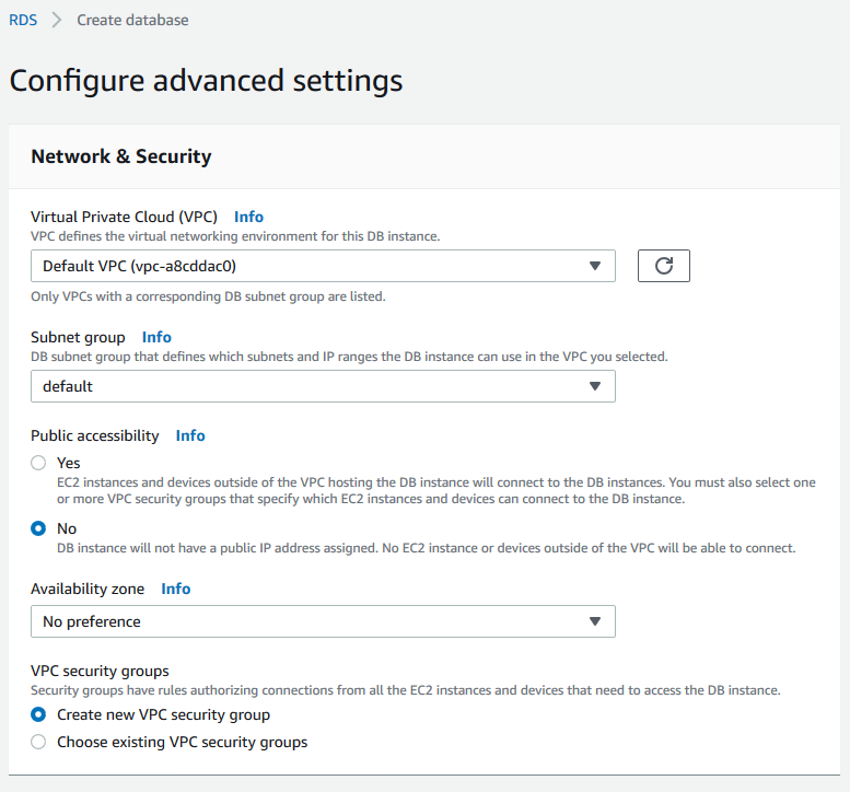
On the Advanced Settings page we’ll configure Network and Security, Windows Authentication, Database Options such as port number, Encryption (where available), Backup retention, Monitoring, Performance Insights, Maintenance options, and Deletion protection. I’m going to choose all the defaults for this post, but this is a page where you want to make sure you choose what is best for your environment.
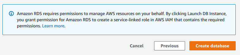
Once you are finished on the Advanced Settings page, click Create Database.
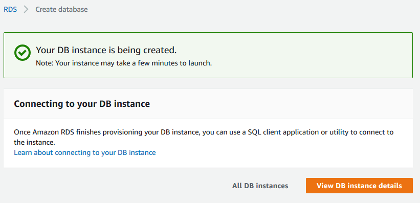
Now how easy was that? Creating a new DB instance took about 2 minutes. Once your instance is created let’s click on View DB Instance details:
The details page gives you all sorts of info about your instance:
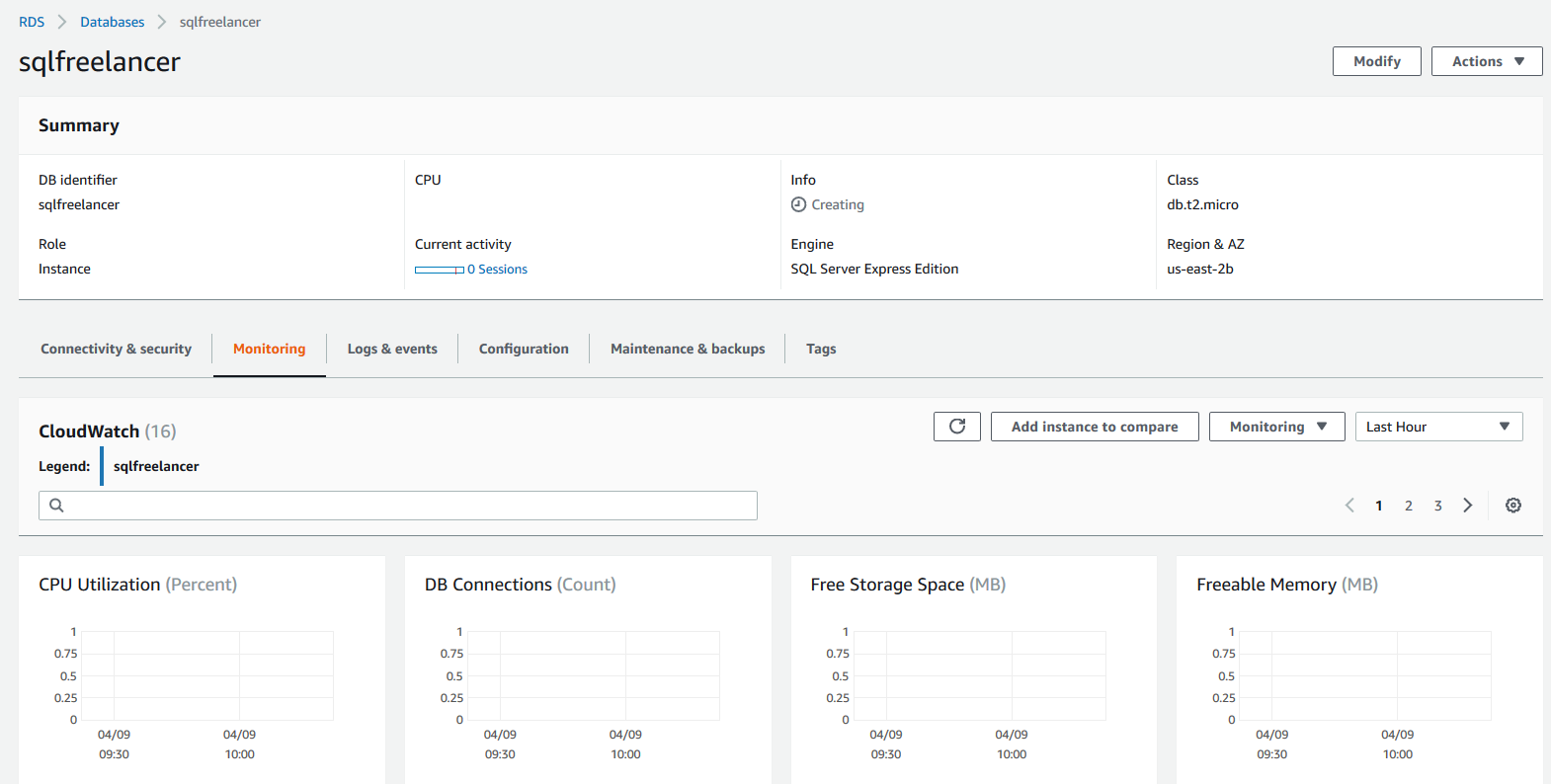

As defined by Amazon, Amazon Relational Database Service (Amazon RDS) makes it easy to set up, operate, and scale a relational database in the cloud. It provides cost-efficient and resizable capacity while automating time-consuming administration tasks such as hardware provisioning, database setup, patching and backups. It frees you to focus on your applications so you can give them the fast performance, high availability, security and compatibility they need.
RDS is also referred to as a Database as a Service (DbaaS) or Platform as a Service (PaaS) not to be confused with Infrastructure as a Service (IaaS) which we’ll discuss in the next paragraph.
DbaaS vs. IaaS
| DbaaS | IaaS |
| You can choose any DB platform such as Oracle, MySQL, SQL Server, Amazon Aurora, PostgreSQL, and MariaDB | You create a Virtual Machine and install OS and DB platform such as SQL Server |
| DbaaS takes care of backups, High Availability, Patching, OS, underlying hardware | Iaas will only take care of the VM host layer and it’s hardware. You will need to manage patching, HA, security, etc. This is essentially like an on premise server. |
Being an Operational DBA, there are a few tasks that RDS will take over freeing up time for the DBA to focus on other things. Some of those tasks include the following:
Wow! All of these items make managing a SQL Server much easier for a DBA right? Do you even need a DBA if you’re running RDS? Of course you do! While it does make some tasks easier for a DBA, RDS will not do the following:
Now that we’ve discussed some of the pros and cons, why do businesses use DbaaS?
The speed of provisioning increases business value because instead of waiting weeks to bring a server online including purchasing software, servers, licenses, managing resources, etc. you can click a few buttons in the Amazon console and have a fresh SQL Server online in a matter of minutes.
The automation of regular tasks means there’s less possibility of human mistake and less hours spent by the admins patching and managing certain parts of the servers, which means no more late nights. Employees can now spend more time query tuning, deploying new functionality, and making sure the performance is the best. All of this leads to increased revenue for the business.
Using bookmarks in Power BI help you capture the currently configured view of a report page, including filtering and the state of visuals, and later let you go back to that state by simply selecting the saved bookmark.
You can also create a collection of bookmarks, arrange them in the order you want, and subsequently step through each bookmark in a presentation to highlight a series of insights, or the story you want to tell with your visuals and reports.
In this post we’ll quickly go over how to create a few bookmarks and view them as a slideshow if you will.
I’m going to use my March Madness Report I created in an earlier post. Once my report is opened in Power BI Desktop, I’m going to click on the View tab in the ribbon and select “Bookmarks Pane”
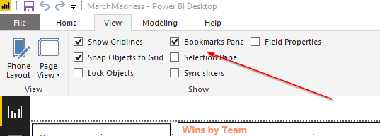
This should bring up a new Bookmarks pane inside PBI Desktop:
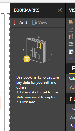
Remember, bookmarks are used to capture the current view of the report so I’m going to use the default view where I’m showing all data and I’m going to name the bookmark “Home”. Make sure all filters are selected to show all data and click Add under the bookmark pane. This will create a new Bookmark, named Bookmark 1. Click the ellipsis and select rename to rename the bookmark appropriately.

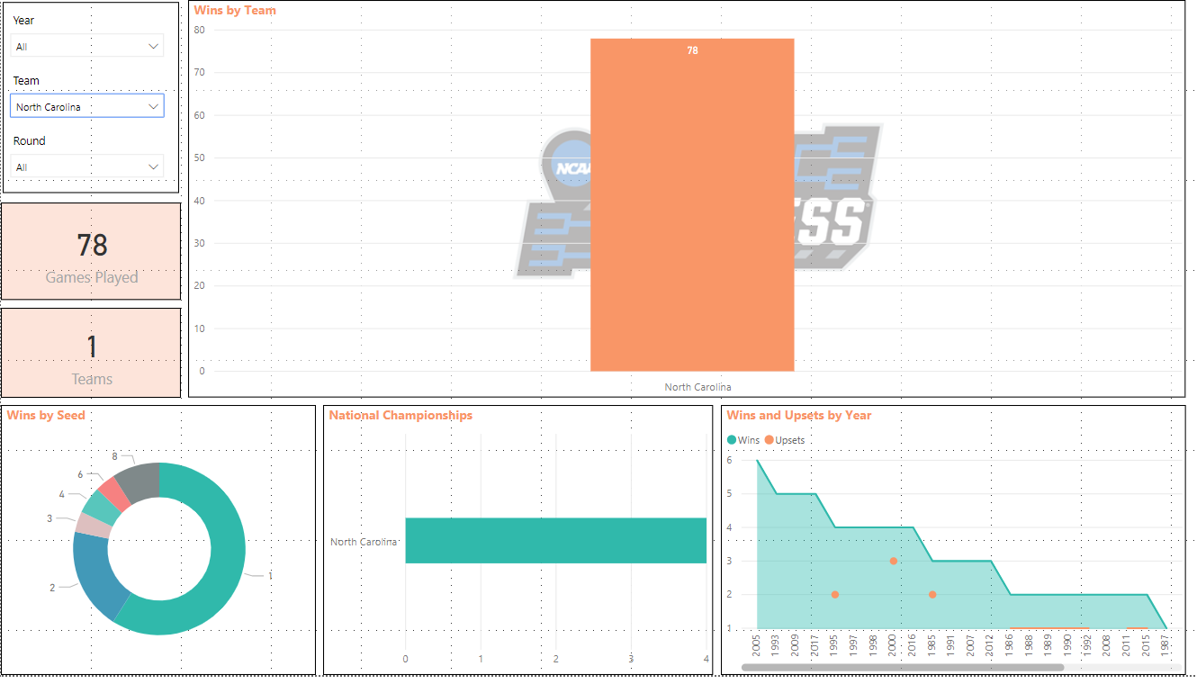
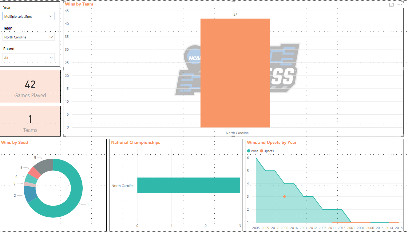
Next, I like North Carolina, so I’m going to go to my Team Filter and choose North Carolina which will show me data for only this team.
In my bookmark pane, I’m going to click Add again and rename to North Carolina.
Next, I want to view data on North Carolina from 2000 to present so I’ll change the Year Filter.
In my bookmark pane, I’m going to click Add again and rename to North Carolina 2000-present.
Now, if I click on any of bookmarks, it will take me to the data that was saved for each. This is a great way to present data in a meeting/conference so you don’t have to manually change the filters during the engagement.
We can also click the View button in the Bookmark pane to view a slideshow using the arrows at the bottom to navigate:

I wrote a post a few weeks about creating an Azure Windows VM so wanted to follow up with a post about creating an AWS Windows VM to compare both platforms. I like Azure and AWS so I’m not going to throw either one under the bus. Both are great and easy to use.
Let’s create an AWS (EC2) Windows VM.
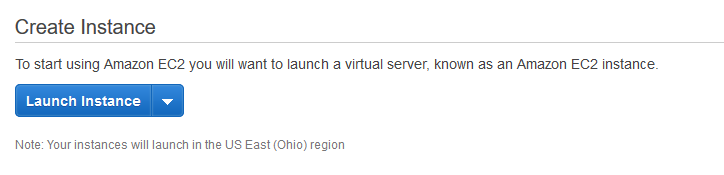
Log into the AWS portal and click on EC2 under All Services, Compute:

Next, click Launch Instance:
Step 1 allows you to choose an Amazon Machine Image or AMI. There are tons of options here, but for this post, I’m going to use Microsoft Windows Server 2019 Base

Once I click Select, I’m brought to Step 2: Choose an Instance Type. Instance Types comprise varying combinations of CPU, memory, storage, and networking capacity and give you the flexibility to choose the appropriate mix of resources for your applications. Each instance type includes one or more instance sizes, allowing you to scale your resources to the requirements of your target workload. More info here: https://aws.amazon.com/ec2/instance-types/
For this post, and for cost sake, I’m going to use the free tier t2.micro type which is 1 CPU, 1GB RAM

Once I’ve selected my instance type I’ll click Next:Configure Instance Details.
Step 3: Configure Instance Details is where we’ll configure our new server. Let’s go down the list.
For this post I’ll use defaults and click Next.
Step 4 is Add Storage.
I’m not going to go over each Storage option, but you can get more info here: https://docs.aws.amazon.com/AWSEC2/latest/UserGuide/Storage.html?icmpid=docs_ec2_console
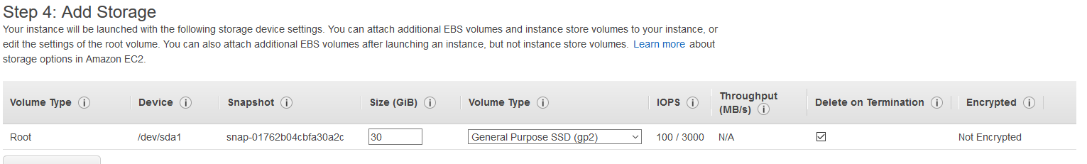
Selecting default and clicking next.
Step 5: Add Tags.
Like Azure, A tag consists of a case-sensitive key-value pair. For example, you could define a tag with key = Name and value = Webserver. A copy of a tag can be applied to volumes, instances or both. Tags will be applied to all instances and volumes
Click Next.
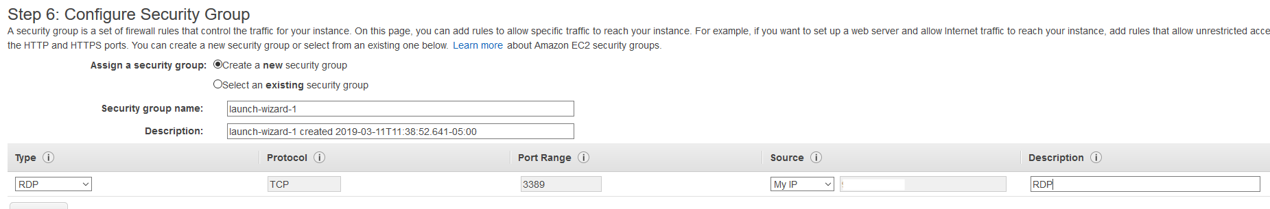
Step 6 is Configure Security Group
A security group is a set of firewall rules that control the traffic for your instance. On this page, you can add rules to allow specific traffic to reach your instance. For example, if you want to set up a web server and allow Internet traffic to reach your instance, add rules that allow unrestricted access to the HTTP and HTTPS ports. By default, the RDP port is added, but it allows all IP addresses to connect. Changing the Source column will allow you to filter what IP’s are able to RDP into the server. For this post, I’m going to change the Source column to allow “My IP”
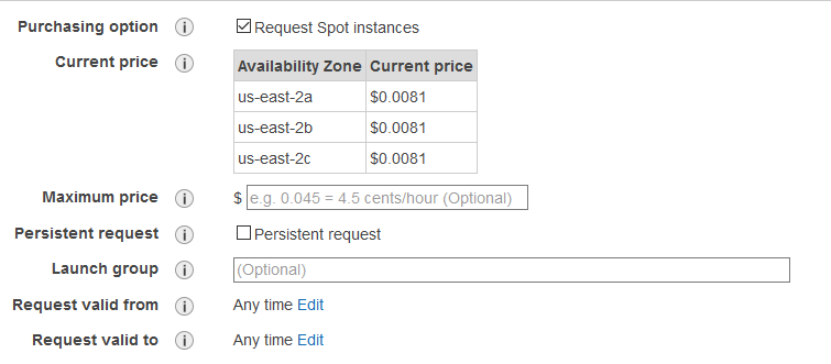
Next…and last page is a summary of the options selected. To finish configuring the instance, click Launch.

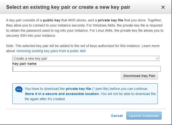
After clicking launch, you will see a popup where you can create or use an existing key pair. A key pair consists of a public key that AWS stores, and a private key file that you store. Together, they allow you to connect to your instance securely. For Windows AMIs, the private key file is required to obtain the password used to log into your instance. For Linux AMIs, the private key file allows you to securely SSH into your instance.
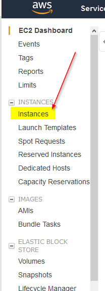
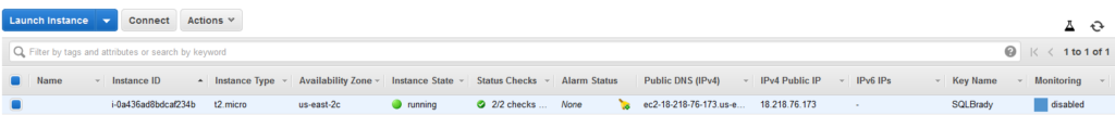
Once the new VM is created, you can go back to the EC2 dashboard and click on Instances to see the new VM:
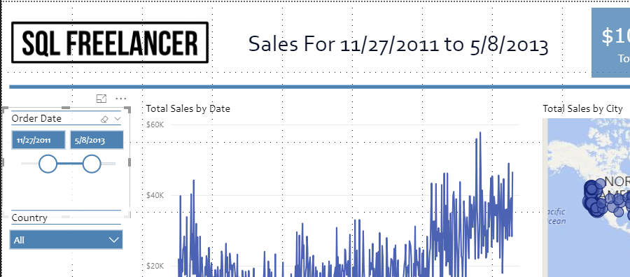
Creating a dynamic title in Power BI helps present the data and let’s the viewers know what the data is filtered on. In this post I’ll go over how to do this…
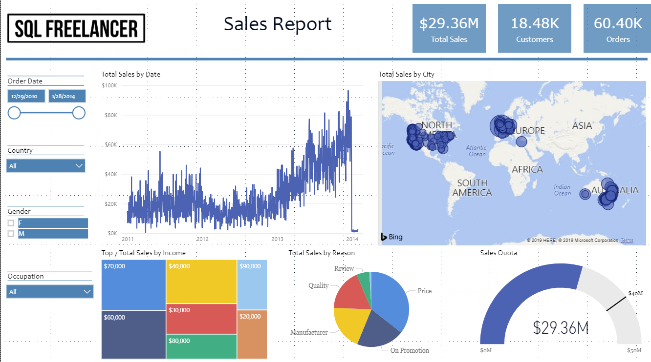
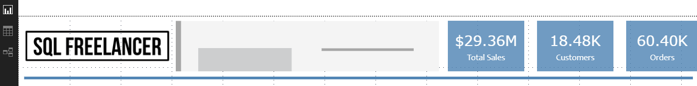
I have a sales report that I’d like to add a title that is based on the Order Date Slicer. Currently, the title is static text “Sales Report”
To create my dynamic title, I’ll first need to create a measure table that has my Order Date data. In this case, that table is FactInternetSales and the column is OrderDate.
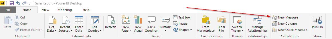
To create a measure, click New Measure in the Power BI Desktop ribbon
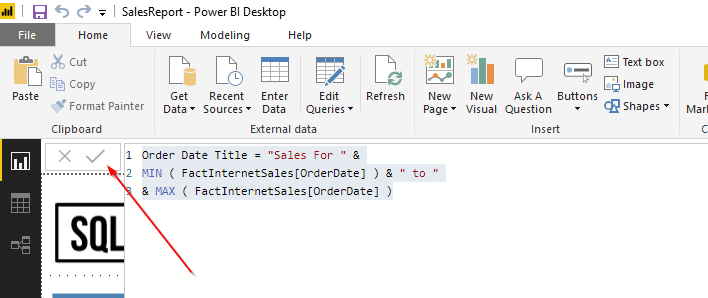
Next, you’ll see a window where you can type code. In this example, I’ll use the following DAX
Next, you’ll see a window where you can type code. In this example, I’ll use the following DAX
Order Date Title = “Sales For ” &
MIN ( FactInternetSales[OrderDate] ) & ” to “
& MAX ( FactInternetSales[OrderDate] )
Let’s walk through this real quick.
The first line (Order Date Title = “Sales For “ &) is basically naming the measure and adding the beginning text for the title.
The second line (MIN ( FactInternetSales[OrderDate] ) & “ to “) is finding the minimum order date from FactInternetSales.OrderDate and then adding the “to” text.
The last line (MAX ( FactInternetSales[OrderDate] ) is finding the maximum order date from FactInternetSales.OrderDate.
This one was pretty easy. Once I’ve typed my DAX, hit the checkmark to make sure there are no errors and the click off screen.
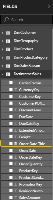
Our measure has been created! Let’s go back and find it under the FactInternetSales fields pane.
Next, let’s click on the Card Visualization and move and size it appropriately to fit in our title space.
While the card is highlighted, click on the new measure from the Fields pane and it will populate the card with the measure we created.
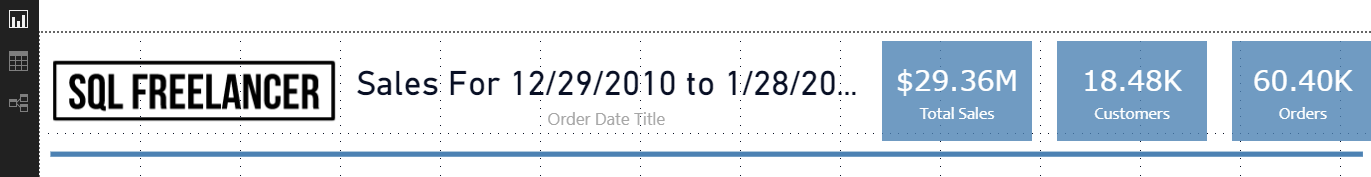
The only thing left to do is format the title and we’re all set! If we change the Order Date Slicer, you’ll notice the title changes with the date. See live example at the beginning of this post.
At the beginning of the year I set a goal to learn something new. I’ve always loved business intelligence and bringing data to life in the form of dashboards and charts so for the 1st half of the year I wanted to focus on Microsoft’s Power BI. I’m not going to explain what Power BI is, but if you want to read up on it go here: https://powerbi.microsoft.com/en-us/
This post is just going to show off my dashboard. ? See live example above.
I’m a huge sports fan and the best time of the year happens to fall in March. Besides my birthday being in March, it’s also March Madness. Hours and hours of basketball. I could of used AdventureWorks for my dataset, but I wanted to use something I’m interested in. I found some data containing every NCAA tournament game result since 1985 (when the tournament was expanded to the 64 team bracket). The dataset contains the year, round (1-6), seed of the teams (1-16), region (1-4) and the scores. Perfect. Let’s use this to create a dashboard.
There’s not a ton of data, but I used what I could and tried to answer some questions around wins and upsets. Here’s a screenshot of the final product:
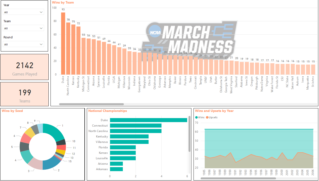
You can see Wins By Team (Duke with 93, North Carolina with 78, etc), Wins by Seed, National Championships, and Upsets vs Wins by Year. You can also see that a total of 2142 games have been played with 199 different teams in the tournament.
This was really fun and answers a lot of the questions I was thinking in my head while designing. The top left corner also has slicers which help filter the data. For example, if I wanted to see only the data for 2015 I could change the Year slicer to 2015 and it would update all my visualizations:

You can see that Duke won the National Championship from the National Championships visualization. If you hover over the Wins and Upsets visualization, you’ll see there were 30 upsets out of 63 games.
Let’s say I want to view data for a certain Team. Let’s choose Alabama Crimson Tide. If I change the Team slicer to Alabama I can see some data based around this team.
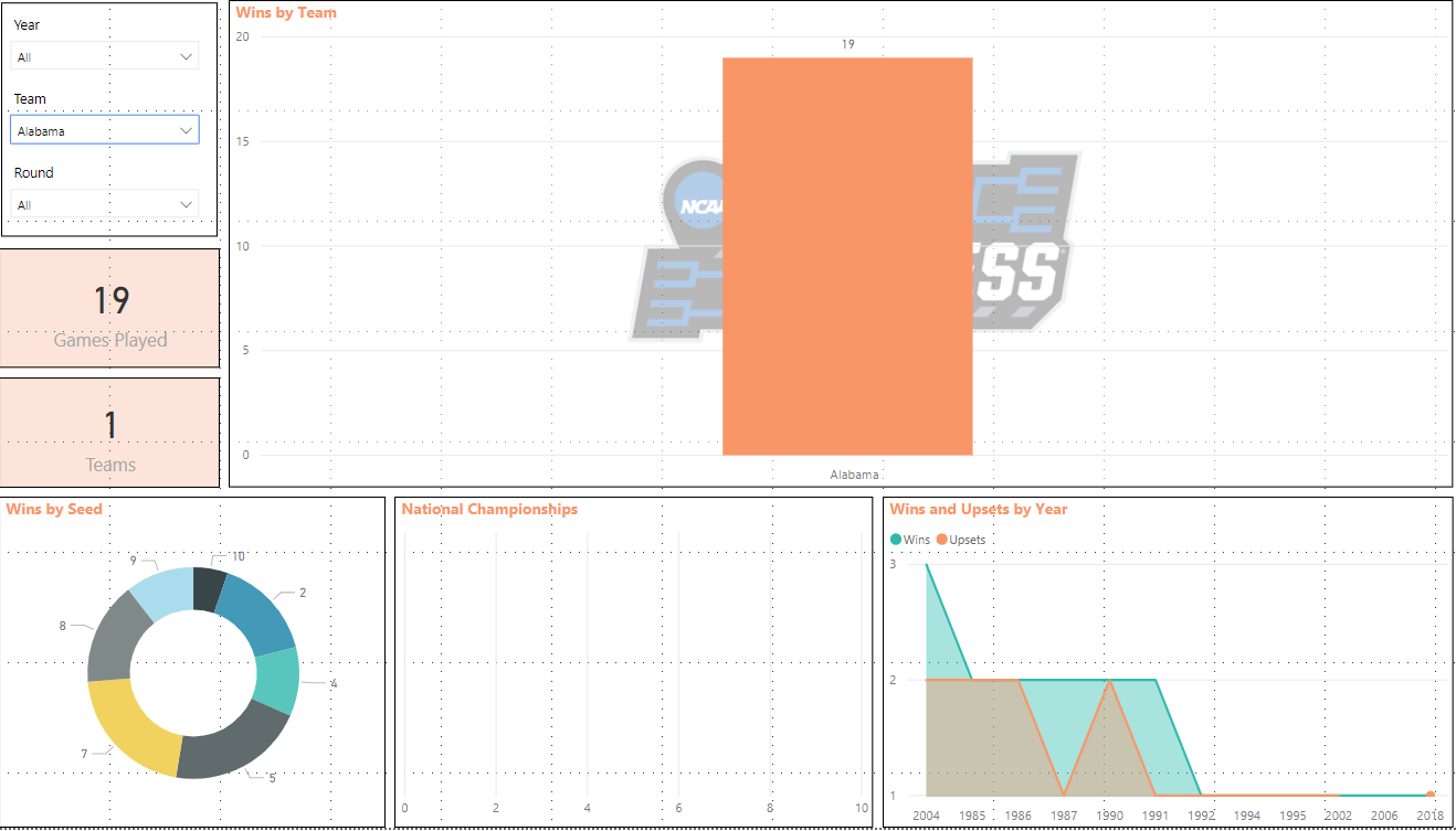
Alabama has won 19 NCAA tournament games, 0 national championships, has been a 5 or 7 seed 21% of the time and they’ve had a few upsets along the way. Not bad for a football school.
What about data for the National Championship game? I can change the Round slicer to 6, which is the National Championship round and view the data this way.
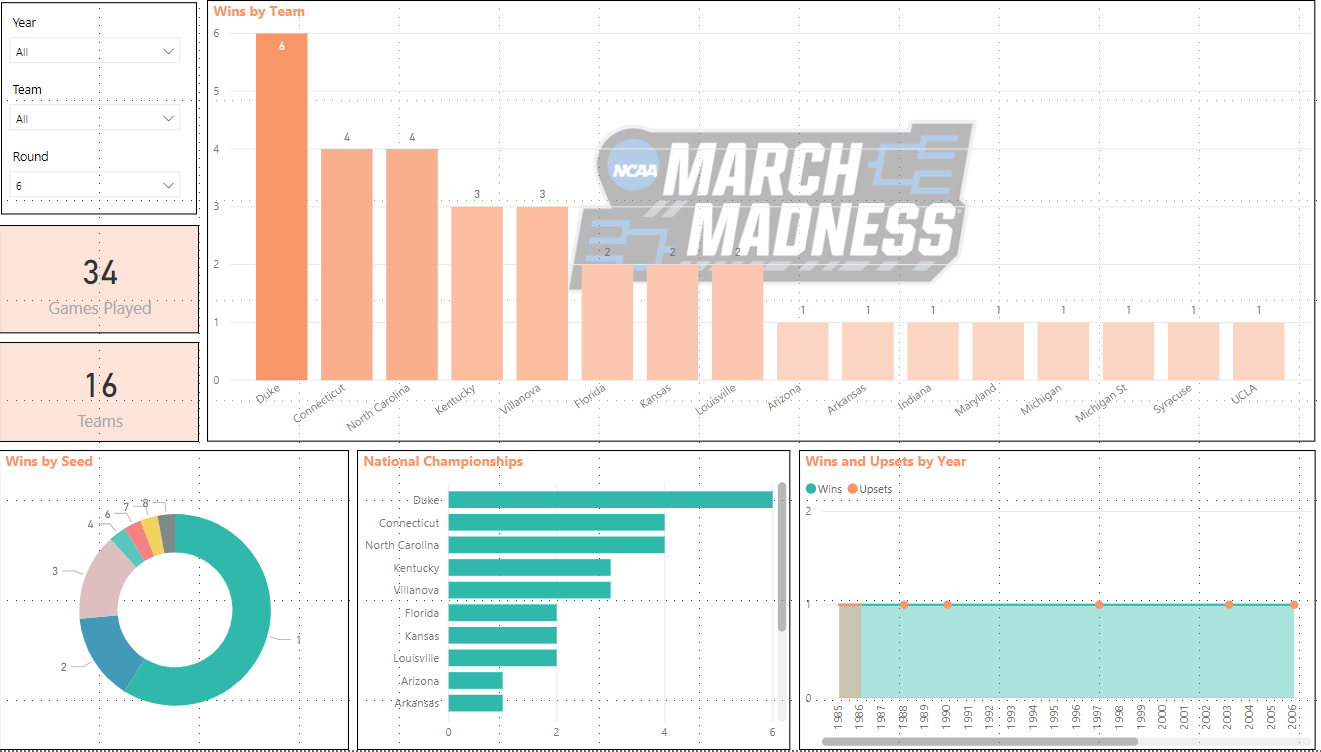
I can see out of 34 games, there has only been 16 different teams make the National Championship. Duke leads the way with 6, followed by North Carolina and Connecticut with 4. The 1 seed has played in this game 59% of the time, and there were upsets in 1988, 1990, 1997, 2003, 2006, and 2016.
We can also click on the visualizations themselves to view data. For example, if we reset our slicers to show all data and click on the #1 seed in the Wins By Seed Donut Chart we see the following:
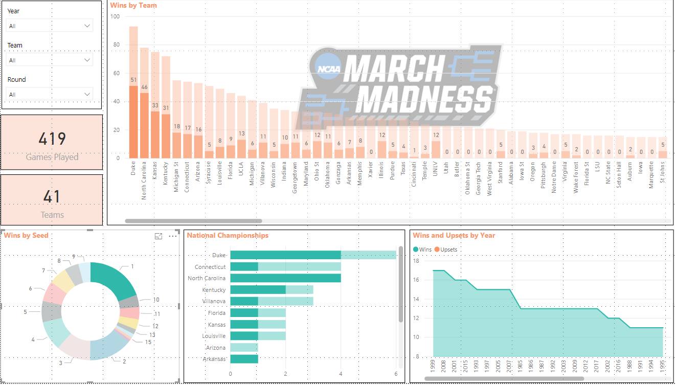
We can see that the #1 seed has played in 419 games with a total of 41 different teams. Duke has won 51 games as the #1 seed while North Carolina has won 46. Duke has also won the National Championship 4 times as the #1 seed and in 1999 the #1 seed won 17 games which is the highest.
Really cool stuff. I loved working on this project and working with this data.
I ran into an issue where SQL Server was installed with the wrong collation and a lot of user databases were already attached. I could easily backup the databases, uninstall, reinstall, and restore the databases back, but this could take literally all day. There is a better and much faster way to make this change. This post will go over it….
First, backup all databases (duh)
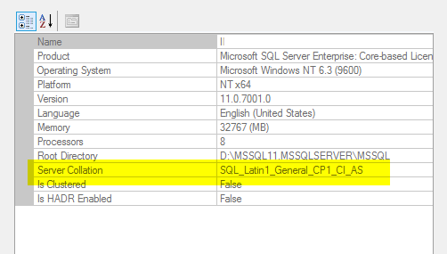
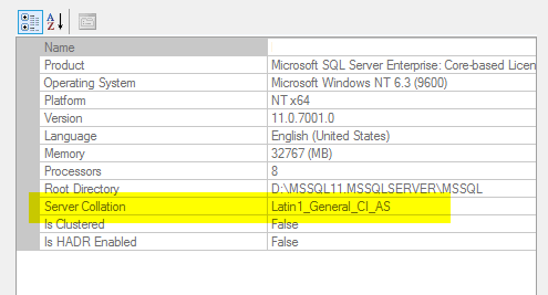
Next, we’ll verify the current collation. On this server it’s set to Latin1_General_CI_AS and I want to change it to SQL_Latin1_General_CP1_CI_AS.
Next, we’ll double check and make sure we have backups of all databases ?
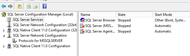
Open SQL Configuration Manager and turn off all SQL Services:
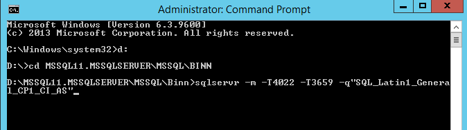
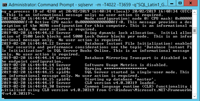
Open Command Prompt (as administrator) and browse to the BINN directory and type the following command.
sqlservr -m -T4022 -T3659 -q”SQL_Latin1_General_CP1_CI_AS”
-m – starts SQL Server in single user admin mode
-T4022 – bypasses all startup procedures
-T3659 – undocument trace flag. enables logging of all errors to the errorlog during startup
-q – new collation
Before hitting Enter, let’s triple check and make sure those backups exist.
Hit Enter.
SQL will run through its startup routine:
Voila. Recovery is complete.
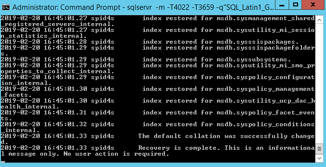
Close Command Prompt and start the SQL services back up.
Back in SQL Server Management Studio, verify that the collation has changed.