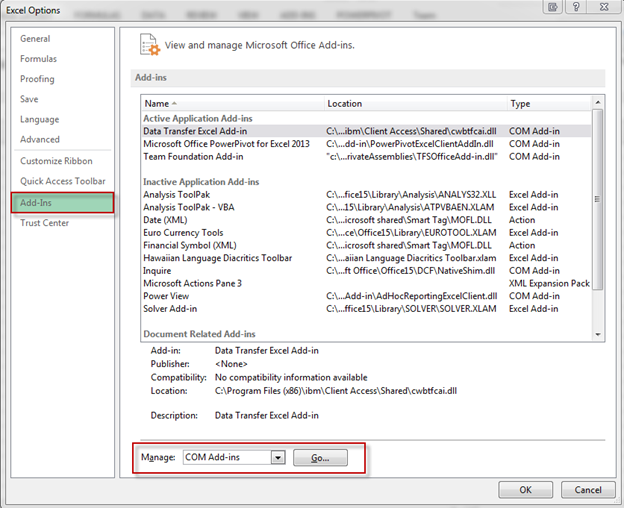
Excel 2013 changes things up a bit when it comes to installing PowerPivot. In previous versions you had to download the component and install, but with Excel 2013 it comes installed as an add-in, but disabled by default. To enable PowerPivot, open Excel, go to File, Options, Add-Ins, select COM Add-ins and click Go.
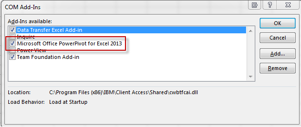
This will open up the COM Add-Ins dialog box. Click “Microsoft Office PowerPivot for Excel 2013” and hit OK.
After successfully enabling PowerPivot, the tab should appear at the top of the Excel spreadsheet.
![]()
Creating a dashboard
There are a few different ways in which to import data into Excel to use with PowerPivot. Some of these ways include:
- From database
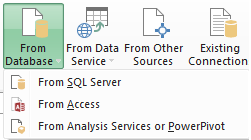
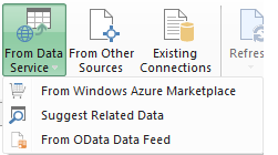
- From Data Service
- From other sources such as Oracle, Excel, flat files, etc.
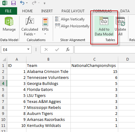
For this example, and simplicity sake, I will just run a query and simply copy and paste my results into the Excel spreadsheet. The query results look like this:

Once the results are copied and pasted into Excel, click the PowerPivot tab and click Add to Data Model:
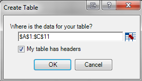
On the create table dialog box, make sure you select the range for your data and click “My table has headers”
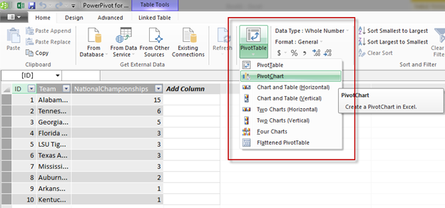
After clicking OK, the PowerPivot window should appear. To start creating the dashboard, click PivotTable, PivotChart, then select New Worksheet: